-
-

Logo!
-

Example of models dictionary in client class with only 1 classification neural network.
-

Output of tune()
-

Sample outfit for generate_fit_cnn() to generate a dataset of apples, oranges, and bananas and train a CNN for it with just 3 epochs.
-
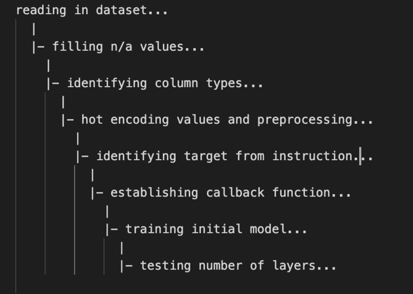
Example process logger
-

Sample of all plots generated for clustering query. Only plots for best cluster are stored.
-

Generated model train vs test accuracy plot for classification neural network query.
-

Example generated clustering plot for n_clusters = 9
-

Similarity Spectrum for stat_analysis()
-

GitHub commit history!


Check out the GitHub page if you'd like to see a working Table of Contents. Devpost disables same-page links so I couldn't get it to work.
Libra: Deep Learning fluent in one-liners
Libra is a machine learning API that allows developers to build and deploy models in fluent one-liners. It is written in Python and TensorFlow and makes training neural networks as simple as a one line function call. It was written to make machine learning as simple as possible for every software developer.
Motivation
With the recent rise of machine learning on the cloud, the developer community has neglected to focus their efforts on creating easy-to-use platforms that exist locally. This is necessary because in a process that has hundreds of API endpoints, it's very difficult to integrate your pre-existing workflow with a cloud based model. Libra makes it very easy to create a model in just one-line, and not have to worry about the specifics and/or the transition to the cloud.
While Keras makes it easy to use Tensorflow's features, it still requires users to understand the basics like how to preprocess his/her dataset, how to build models for his/her task, and architectures for his/her networks. Libra takes all of this out of the hands of the developer, so that the user has to have no knowledge about machine learning in order to create and train models.
Guiding Principles
Beginner Friendly. Libra is an API designed to be used by developers with no deep learning experience whatsoever. It is built so that users with no knowledge in preprocessing, modeling, or tuning can build high-performance models with ease without worrying about the details of implementation.
Quick Integration. With the recent rise of machine learning on the cloud, the developer community has failed to make easy-to-use platforms that exist locally and integrate directly into workflows. Libra allows users to develop models directly in programs with hundreds of API endpoints without having to worry about the transition to the cloud.
Automation. End-to-end pipelines containing hundreds of processes are automatically run for the user. The developer only has to consider what they want to accomplish from the task and the location of their initial dataset.
Easy Extensibility. Queries are split into standalone modules. Under the dev-pipeline module you can pipeline both different and new modules and integrate them into the workflow directly. This allows newly developed features to be easily tested before integrating them into the main program.
Overview
Libra is split up into several main components:
- Client: the client object is where all models and information generated are stored for usage.
- Queries: How models are built and trained in Libra. They're called on client objects and are given an instruction. ALL preprocessing is handled by the queries!
- Image generation: For generating datasets and fitting them to convolutional neural networks automatically.
- Model Information: How to retrieve generated plots, and deep-tune models.
- Dimensionality Reduction: How to perform reduction and feature selection to your dataset easily.
- Process Logger: Keeping track of processes Libra is running in the background.
- Pipelining for contributors: Special module pipeline in order to contribute to Libra.
- User instruction identification: How Libra uses user instruction to determine targets and make predictions.
Table of Contents
- Prediction Queries: building blocks
- Image Generation
- Model Information
- Dimensionality Reduction
- Process Logger
- Pipelining for Contributors
- Providing Instructions
- What's next for Libra?
- Contact
Queries
Queries are how you create and train machine learning algorithms in Libra.
Generally, all queries have the same structure. You should always be passing an English instruction to the query. The information that you generate from the query will always be stored in the clientclass in the model's dictionary. When you call a query on the client object, an instruction will be passed. Any format will be decoded, but avoiding more complex sentence structures will yield better results. If you already know the exact target class label name, you can also provide it.
Regression Neural Network
Let's start with the most basic query. This will build a feed-forward network for a continuous label that you specify.
newClient = client('dataset')
newClient.regression_query_ann('Model the median house value')
No preprocessing is neccesary. All plots, losses, and models are stored in the models field in the client class. This will be explained in the Model Information section.
Basic tuning with the number of layers is done when you call this query. If you'd like to tune more in depth you can call:
newClient.tune('regression', inplace = False)
To specify which model to tune, you must pass the type of model that you'd like to perform tuning on.
This function tunes hyperparameters like node count, layer count, learning rate, and other features. This will return the best network and if inplace = True it will replace the old model it in the client class under regression_ANN.
Now, if I want to use my model, I can do:
newClient.models['regression_ANN'].predict(new_data)
Classification Neural Network
This query will build a feed-forward neural network for a classification task. As such, your label must be a discrete variable.
newClient = client('dataset')
newClient.classification_query_ann('Predict building name')
This creates a neural network to predict building names given your dataset. Any number of classes will work for this query. By default, categorical_crossentropy and an adam optimizer are used.
Convolutional Neural Network
Creating a convolutional neural network for a dataset you already have created is as simple as:
newClient = client()
newClient.convolutional_query('path_to_class1', 'path_to_class2', 'path_to_class3')
For this query, no initial shallow tuning is performed is done because of how memory intensive CNN's can be. User specified parameters for this query are currently being implemented. The defaults can be found in the predictionQueries.py file.
K-means Clustering
This query will create a k-means clustering algorithm trained on your processed dataset.
newClient = client('dataset')
newClient.kmeans_clustering_query()
It continues to grow the number of clusters until the value of inertia stops decreasing by at least 1000 units. This is a threshold determined based on several papers, and extensive testing. This can also be changed by specifying threshold = new_threshold_num. If you'd like to specify the number of clusters you'd like it to use you can do clusters = number_of_clusters.
Nearest-neighbors
This query will use scikit-learn's nearest-neighbor function to return the best nearest neighbor model on the dataset.
newClient = client('dataset')
newClient.nearest_neighbor_query()
You can specify the min_neighbors, max_neighbors as keyword arguments to the function. Values are stored under the nearest_neighbor field in the model dictionary.
Support Vector Machine
This will use scikit-learn's SVM function to return the best support vector machine on the dataset.
newClient = client('dataset')
newClient.svm_query('Model the value of houses')
Values are stored under the svm field in the model dictionary.
NOTE: A linear kernel is used as the default, this can be modified by specifying your new kernel name as a keyword argument: kernel = 'rbf_kernel'.
Decision Tree
This will use scikit's learns decision tree function to return the best decision tree on the dataset.
newClient = client('dataset')
newClient.decision_tree_query()
This will use scikit's learns Decision Tree function to return the best decision tree on the dataset. Values are stored under the decision_tree field in the model dictionary.
You can specify these hyperparameters by passing them as keyword arguments to the query: max_depth = num, min_samples_split = num, max_samples_split = num, min_samples_leaf = num, max_samples_leaf= num
Image Generation
Class wise image generation
If you want to generate an image dataset to use in one of your models you can do:
generate_set('apples', 'oranges', 'bananas', 'pineapples')
This will create separate folders in your directory with each of these names with ~100 images for each class. An updated version of Google Chrome is required for this feature; if you'd like to use it with an older version of Chrome please install the appropriate chromedriver.
Generate Dataset and Convolutional Neural Network
If you'd like to generate images and fit it automatically to a Convolutional Neural Network you can use this command:
newClient.generate_fit_cnn('apples', 'oranges')
This particular will generate a dataset of apples and oranges by parsing Google Images, preprocess the dataset appropriately and then fit it to a convolutional neural network. All images are reduced to a standard (224, 224, 3) size using a traditional OpenCV resizing algorithm. Default size is the number of images in one Google Images page before having to hit more images, which is generally around 80-100 images.
The infrastructure to generate more images is currently being worked on.
Note: all images will be resized to (224, 224, 3). Properties are maintained by using a geometric image transformation explained here: OpenCV Transformation.
Model Modifications
Model Tuning
In order to further tune your neural network models, you can call:
newClient.tune('convolutional neural network')
This will tune:
- Number of Layers
- Number of Nodes in every layer
- Learning Rate
- Activation Functions
In order to ensure that the tuned models accuracy is robust, every model is run multiple times and the accuracies are averaged. This ensures that the model configuration is optimal.
You can just specify what type of network you want to tune — it will identify your target model from the models dictionary using another instruction algorithm.
NOTE: Tuning for CNN's is very memory intensive, and should not be done frequently.
Plotting
All plots are stored during runtime. This function plots all generated graphs for your current client object on one pane.
newClient.plot_all('regression')
If you'd like to extract a single plot, you can do:
newClient.show_plots('regression')
and then
newClient.getModels()['regression']['plots']['trainlossvstestloss']
No other plot retrieval technique is currently implemented. While indexing nested dictionaries might seem tedious, this was allowed for fluency.
Dataset Information
In depth metrics about your dataset and similarity information can be generated by calling:
newClient.stat_analysis()
A information graph as well as a similarity spectrum shown below will be generated. This can be found in the image gallery under "Similarity Spectrum."
This represents 5 columns that have the smallest cosine distance; you might need to remove these columns because they're too similar to each other and will just act as noise. You can specify whether you want to remove them with inplace = True. Information on cosine similarity can be found here.
If you'd like information on just one column you can do:
newClient.stat_analysis(dataset[column_name])
Dimensionality Reduction
Reduction Pipeliner
If you'd like to get the best pipeline for dimensionality reduction you can call:
dimensionality_reduc(I want to estimate the number of households', path_to_dataset)

or

newClient.dimensionality_reducer(I want to estimate the number of households')
Instructions like "I want to model x" are provided in the dimensionality reduction pipeline because it identifies which prediction objective you would like to maximize the accuracy for. Providing this instruction helps Libra provide users with the best modification pipeline.
Libra current supports feature importance identification using random forest regressor, indepedent component analysis, and principle component analysis. The output of the dimensionalityReduc() function should look something like this:
Baseline Accuracy: 0.9752906976744186
----------------------------
Permutation --> ('RF',) | Final Accuracy --> 0.9791666666666666
Permutation --> ('PCA',) | Final Accuracy --> 0.8015988372093024
Permutation --> ('ICA',) | Final Accuracy --> 0.8827519379844961
Permutation --> ('RF', 'PCA') | Final Accuracy --> 0.3316375968992248
Permutation --> ('RF', 'ICA') | Final Accuracy --> 0.31419573643410853
Permutation --> ('PCA', 'RF') | Final Accuracy --> 0.7996608527131783
Permutation --> ('PCA', 'ICA') | Final Accuracy --> 0.8832364341085271
Permutation --> ('ICA', 'RF') | Final Accuracy --> 0.8873546511627907
Permutation --> ('ICA', 'PCA') | Final Accuracy --> 0.7737403100775194
Permutation --> ('RF', 'PCA', 'ICA') | Final Accuracy --> 0.32630813953488375
Permutation --> ('RF', 'ICA', 'PCA') | Final Accuracy --> 0.30886627906976744
Permutation --> ('PCA', 'RF', 'ICA') | Final Accuracy --> 0.311531007751938
Permutation --> ('PCA', 'ICA', 'RF') | Final Accuracy --> 0.8924418604651163
Permutation --> ('ICA', 'RF', 'PCA') | Final Accuracy --> 0.34205426356589147
Permutation --> ('ICA', 'PCA', 'RF') | Final Accuracy --> 0.9970639534883721

Best Accuracies
----------------------------
["Permutation --> ('ICA', 'PCA', 'RF) | Final Accuracy --> 0.9970639534883721"]
The baseline accuracy represents the accuracy acheived without any dimensionality reduction techniques. Then, each possible reduction technique permutation is displayed with its respective accuracy. At the bottom is the pipeline which resulted in the highest accuracy. You can also specify which of the reduction techniques you'd like to try by passing reducers= ['ICA', 'RF'] to the function.
If you'd like to replace the dataset with one that replaces it with the best reduced one, you can just specify inplace=True.
Principle Component Analysis
Performing Principle Component is as simple as:
dimensionality_PCA("Estimating median house value", path_to_dataset)
NOTE: this will select the optimal number of principal components to keep. The default search space is up to the number of columns in your dataset. If you'd like to specify the number of components you can just do n_components = number_of_components.
Feature Importances via Random Forest Regressor
Using the random forest regressor to identify feature importances is as easy as calling:
dimensionality_RF("Estimating median house value", path_to_dataset)
This will find the optimal number of features to use and will return the dataset with the best accuracy. If you'd like to manually set the number of feature you can do n_features = number of features.
Indepedent Component Analysis
Performing Indepedent Component Analysis can be done by calling:
dimensionality_ICA("Estimating median house value", path_to_dataset)
If this does not converge a message will be displayed for users to warn them by default.
Process Logger
Libra will automatically output the current process running in a hierarchial format like this:
loading dataset...
  |
  |- getting most similar column from instruction...
    |
    |- generating dimensionality permutations...
      |
      |- running each possible permutation...
        |
        |- realigning tensors...
          |
          |- getting best accuracies...
A quiet mode feature is currently being implemented.
Pipelining for Contributors
In order to help make Libra extensible, a process pipeliner has been implemented to help contributors easily test their newly-developed modules.
Let's say you've developed a different preprocesser for data that you want to test before integrating it into Libra's primary workflow. This is the process to test it out:
First, you want to initialize your base parameters, which are your instructions, the path to your dataset, and any other information your new function might require.
init_params = {
    'instruction': "Predict median house value",
    'path_to_set': './data/housing.csv',
}
You can then modify the main pipeline:
single_regression_pipeline = [initializer,
                your_own_preprocessor, #is originally just preprocessor
                instruction_identifier,
                set_splitter,
                modeler,
                plotter]
These pipelines can be found under the dev-pipeliner folder. Currently, this format is only supported for the single regression pipeline. Complete integration of pipelining into the main framework is currently being implemented.
Finally, you can run your pipeline by using:
[func(init_params) for func in reg_pipeline]
All model information should be stored in init_params. If you'd like to modify smaller details, you can copy over the module and modify the smaller detail; this split was not done to maintain ease of use of the pipeline.
Instructions
newClient.svm_query('Estimate household value') --> target: households, found similar in dataset ✓
Libra uses intelligent natural language processing to analyze user instructions and match it with a column in the users dataset.
- Textblob, a part of speech recognition algorithm, is used to identify parts of speech.
- A self-developed part-of-speech deciphering algorithm is used to extract relevant parts of a sentence.
- Masks are generated to represent all words as tensors in order for easy comparison
- Levenshentein distances are used to match relevant parts of the sentence to a column name.
- Target column selected based on lowest levenshentein distance and is returned.
What's next for Libra
- Q-learning and Policy Gradient Queries
- Make process pipeline part of main framework
- Modularize the data preprocessor for structured data
- Data Augmentation queries
- Sentiment Analysis
Contact
If you're excited about Libra and are looking to contribute please reach out to me via email or linkedin to get started with onboarding. This will begin after this hackathon is completed.
Email: ps9cmk@virginia.edu Linkedin: https://www.linkedin.com/in/palash-sh/
Responsible AI considerations are attached as a Google Docs link below.


Log in or sign up for Devpost to join the conversation.