Inspiration: The Quest for the Third Dimension
In numerical optimization for deep learning, we have long been confined to the first and second dimensions.
- First-order optimizers (e.g., SGD, AdamW) evaluate the gradient vector $g = \nabla L(\theta) \in \mathbb{R}^n$, showing us the direction of steepest descent (a 1D representation).
- Second-order optimizers (e.g., AdaHessian, Sophia, L-BFGS) approximate the Hessian matrix $H = \nabla^2 L(\theta) \in \mathbb{R}^{n \times n}$, adjusting our steps based on local curvature (a 2D representation).
This naturally led us to a simple, ambitious question: What if we make a third-order optimizer?
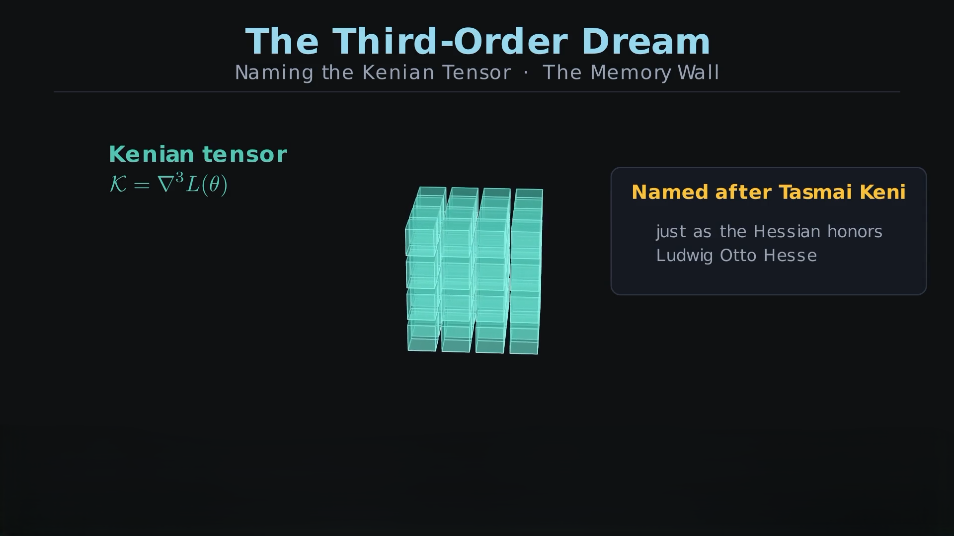
A third-order optimizer would utilize the third-derivative tensor $\mathcal{K} = \nabla^3 L(\theta) \in \mathbb{R}^{n \times n \times n}$. We call this 3D tensor the "Kenian" tensor, named after Tasmai Keni (just as the 2D tensor is named after Ludwig Otto Hesse).
However, directly computing or storing the Kenian tensor is next to impossible. For a modern neural network with even a modest number of parameters, say $n = 39 \times 10^6$ (39 million), the Kenian tensor would require: [ n^3 = (39 \times 10^6)^3 \approx 5.9 \times 10^{22} \text{ elements} ] Storing this in 32-bit floating point precision would require approximately $2.37 \times 10^{14}$ gigabytes (or 237,000 exabytes) of memory. This represents a brick wall of $O(n^3)$ space and computational complexity that makes naive third-order optimization completely impractical.
The Innovation: Trajectory Slicing
To bypass this $O(n^3)$ bottleneck, we realized that we do not need the full Kenian tensor. We only need the specific direction in which the optimizer is actually moving.
Every step, the optimizer determines a base update direction $\Delta_0$ (our AdamW step). Instead of evaluating the entire tensor $\mathcal{K}$, we only evaluate the exact directional third-order slice contracted along $\Delta_0$: [ \kappa = \mathcal{K}\left[\frac{\Delta_0}{|\Delta_0|_2}, \frac{\Delta_0}{|\Delta_0|_2}, \cdot\right] = \nabla^3 L(\theta)[u, u, \cdot] ] where $u = \frac{\Delta_0}{|\Delta_0|_2}$ is the normalized update direction. This contractive slice $\kappa \in \mathbb{R}^n$ has the same dimensionality as our gradient vector ($O(n)$ space complexity), requiring only a fraction of a megabyte to store!
We compute this slice exactly using PyTorch's auto-differentiation graph in just two additional reverse-mode passes:
- First Contraction: Compute the scalar projection of the gradient along the normalized direction: [ c_1(\theta) = \langle \nabla L(\theta), u \rangle ]
- Hessian-Vector Product: Differentiate $c_1$ with respect to $\theta$ to obtain the directional second derivative: [ g_1(\theta) = \nabla_\theta c_1(\theta) = \nabla^2 L(\theta) \cdot u ]
- Second Contraction: Compute the scalar projection of $g_1$ along $u$: [ c_2(\theta) = \langle g_1(\theta), u \rangle = u^T \nabla^2 L(\theta) u ]
- Third-Order Slice: Differentiate $c_2$ with respect to $\theta$ to get the final third-order trajectory slice: [ g_2(\theta) = \nabla_\theta c_2(\theta) = \nabla^3 L(\theta)[u, u, \cdot] ]
By keeping an Exponential Moving Average (EMA) of this slice, $\hat{\kappa}$, we obtain a continuous estimation of how the local curvature changes along our trajectory.
The Kenian Update Rule
Using the trajectory slice, we apply a Chebyshev-style third-order correction to the base AdamW step $\Delta_0$. In an idealized cubic model, the gradient residual at the newton step $\Delta_0$ is exactly $\frac{1}{2} \mathcal{K}[\Delta_0, \Delta_0, \cdot]$. Compensating for this gives the corrected update: [ \Delta = \Delta_0 - s \frac{\hat{\kappa}}{D} ] where $D = \sqrt{\hat{v}_t} + \epsilon$ is the AdamW diagonal preconditioner (denominator), and $s$ is a scaling factor.
To prevent the third-order correction from destabilizing training in stochastic, non-convex environments, we enforce a strict preconditioned global cap: [ |\Delta - \Delta_0|_D \le \text{correction_cap} \cdot |\Delta_0|_D ] where the preconditioned norm is defined as $|x|_D = \sqrt{\sum x_i^2 D_i}$. By scaling the correction to fit this cap, we guarantee that the third-order term behaves as a stabilizer and refinement, rather than a wild perturbation.
How We Built It & Agentic Co-pilot
I guided the project with high-level conceptual ideas and mathematical intuitions, while GPT-5.6 Sol on Ultra acted as an autonomous agentic partner, executing the heavy lifting across three dimensions:
- PyTorch Reference & Fused Kernels: Building the reference implementation alongside high-performance elementwise updates written in Triton and custom CUDA to eliminate GPU memory bandwidth bottlenecks.
- Formal Verification in Lean 4: Formally proving our mathematical identities, Chebyshev bounds, and Taylor expansion error residuals in Lean 4 (located in
lean/). - Scientific Honesty & Empirical Validation: GPT-5.6 Sol conducted multi-seed benchmark sweeps with zero hallucination. Crucially, it provided unvarnished, accurate empirical feedback—faithfully reporting that while Kenian won decisively on Vision Transformers ($3.067$ vs $3.135$), it underperformed on Language Transformers ($3.212$ vs $3.182$). This scientific integrity allowed us to diagnose why text noise dominates 3rd-order curvature and propose a signal-quality gate for future work.
Challenges & Learnings
Our experimental results revealed a fascinating dichotomy:
- Vision (ViT on CIFAR-100): Kenian achieved a lower mean validation loss than AdamW ($3.067 \pm 0.013$ vs $3.135 \pm 0.023$) over three seeds. The third-order slice was stable, providing helpful curvature corrections.
- Language (Transformer on WikiText-103): Kenian performed slightly worse than AdamW ($3.212 \pm 0.006$ vs $3.182 \pm 0.003$). The trajectory slice was close to zero for most of training, yet the stochastic updates introduced noise that degraded performance.
Our key learning: High-order directional derivatives can be computed efficiently without $O(n^3)$ space complexity, but their utility depends heavily on the data landscape. In discrete text domains, noise dominates the curvature signal. The next step is developing a signal-quality gate that automatically disables the correction when the signal-to-noise ratio is too low.
Built With
- autodiff
- c++
- cuda
- deep-learning
- formal-verification
- gpu-kernels
- high-performance-computing
- lean4
- mathematical-optimization
- natural-language-processing
- numerical-analysis
- python
- pytorch
- vision-transformer


Log in or sign up for Devpost to join the conversation.