-
-

Interactive Stock Theory Lab LOGO
-
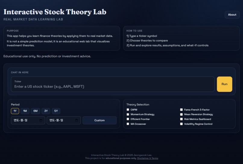
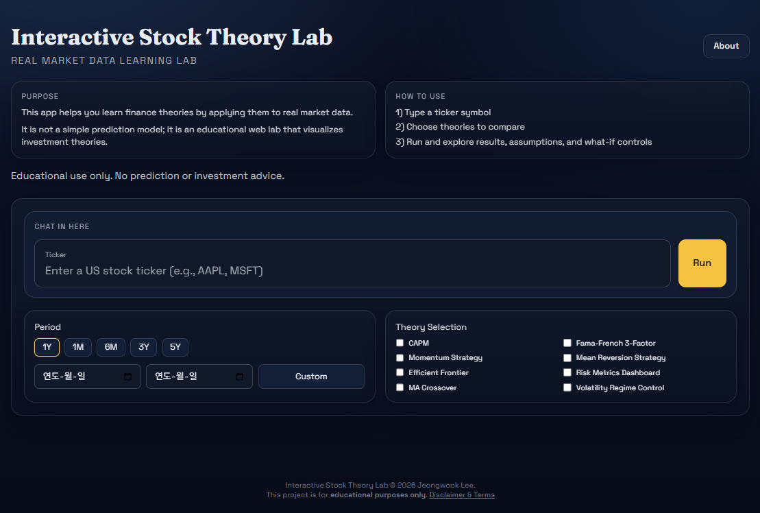
Main First Access Page
-
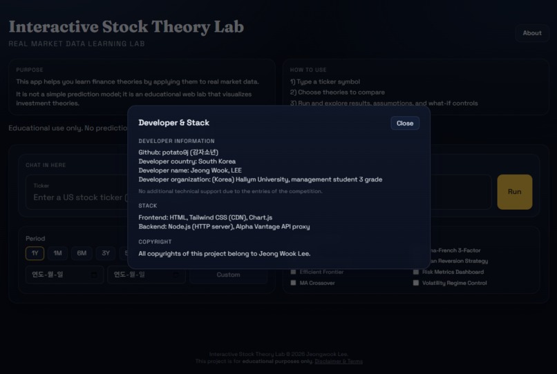
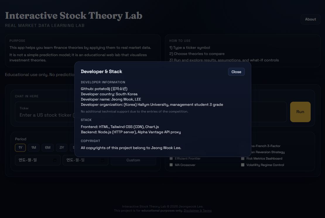
Introducing Developers and Stack
-
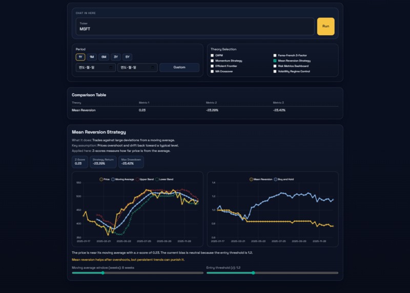
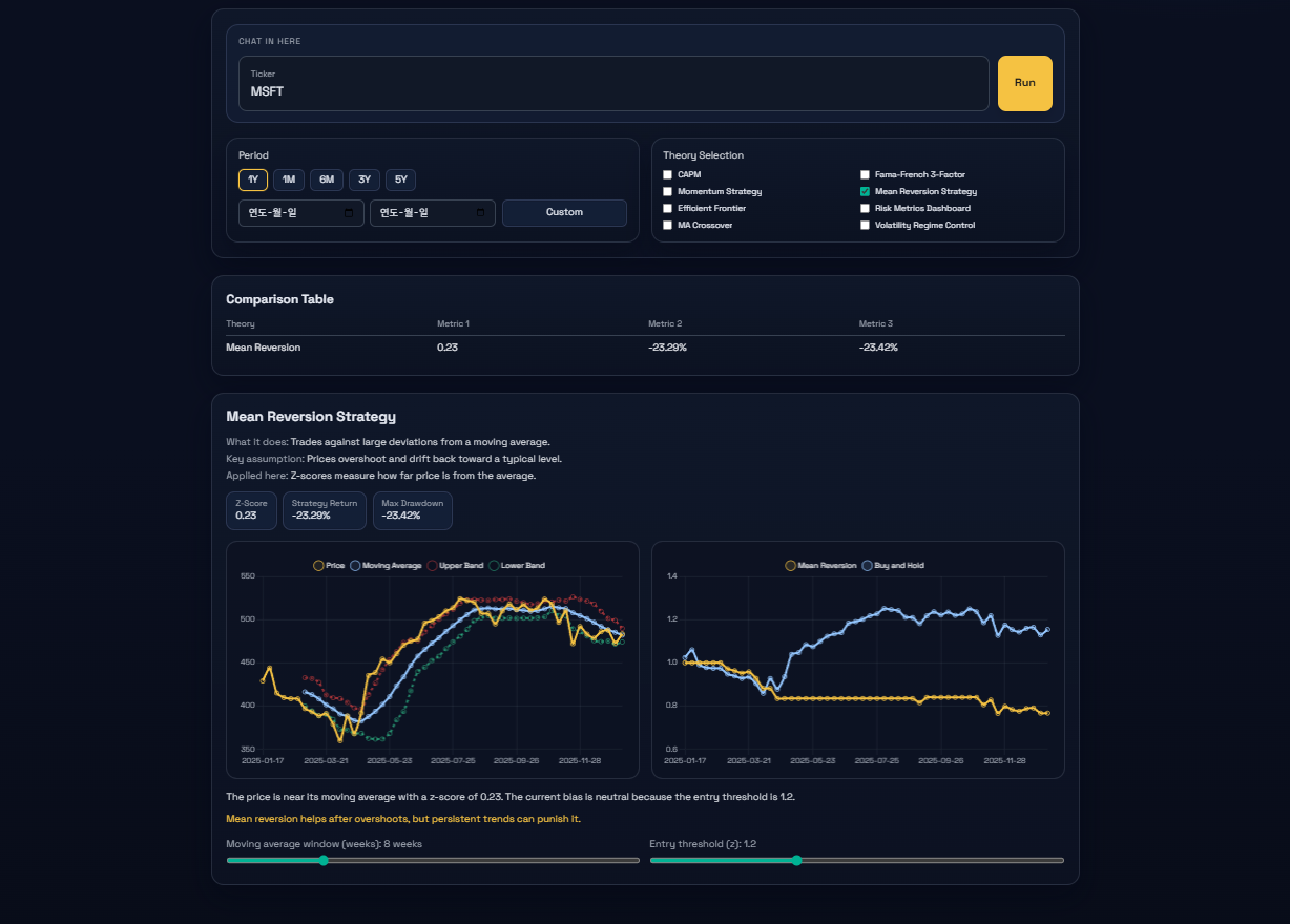
Results window when ticker is entered and theory is selected and executed
-

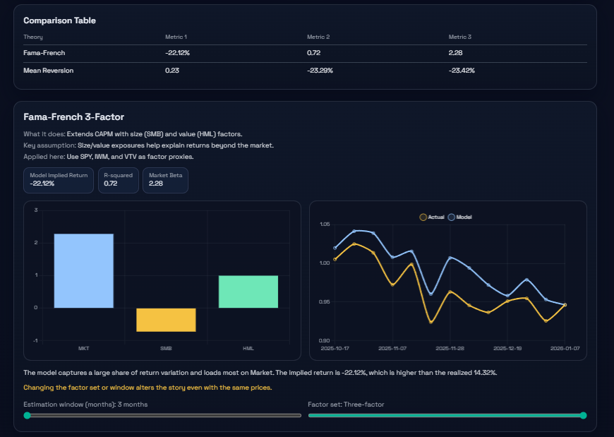
Results window when the Fama-French 3-Factor theory is selected and the Eatification Window value is set to 0
-

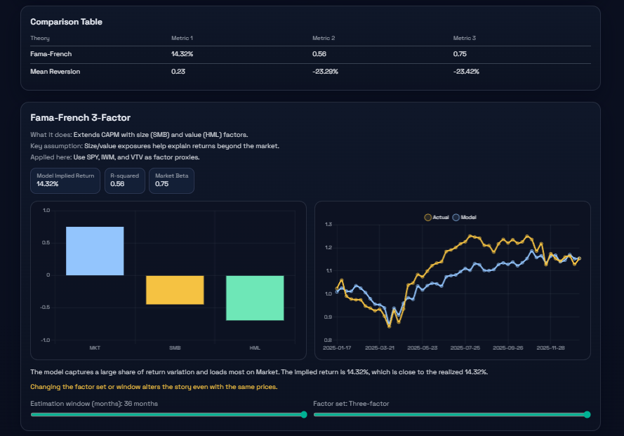
Results window when the Fama-French 3-Factor theory is selected and the Eatification Window value is set to 100
-
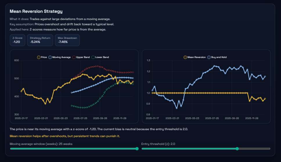
Select Mean Reversion Strategy theory for MSTF ticker and set average window (weeks) to Max, result window
-
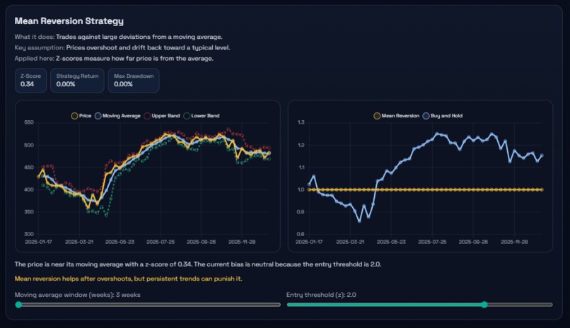
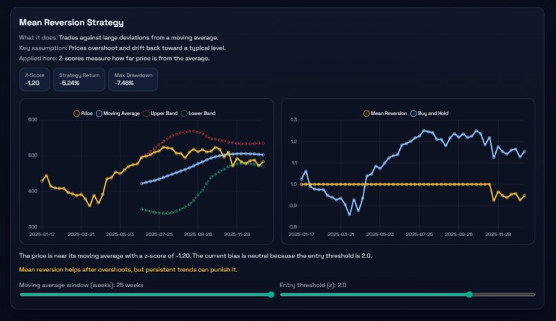
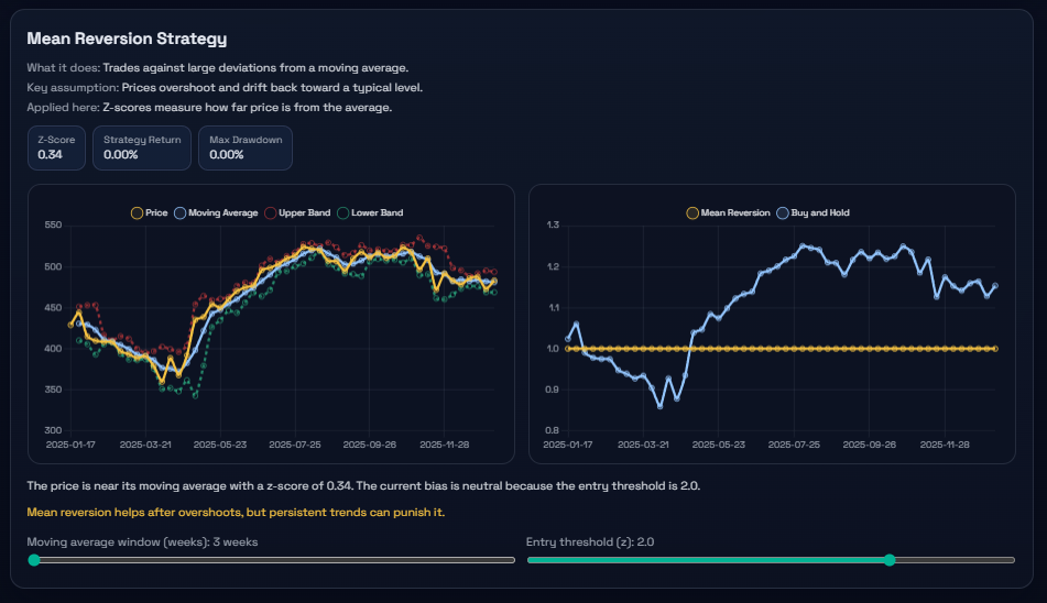
Select Mean Reversion Strategy theory for MSTF ticker and set average window (weeks) to Min, result window

Project Story - Interactive Stock Theory Lab
This document summarizes the project story for the Hackonomics 2026 hackathon. The core goal is understanding, not prediction, by applying finance theories to real market data.
My English is not good. I did my best, but if you find any grammatical errors, I would appreciate it if you could see them as the sweat of Korean college students' hard work.
Inspiration
I am a third-year undergraduate student at Hallym University in South Korea, majoring in Business Administration with double majors in Finance and Big Data. When I studied finance, I focused on formulas and theory from financial engineering, but I struggled to understand how those ideas behave on real data. I believed there were many students like me, so I chose an educational web project to help learners move beyond theory-only study.
What it does
- Users enter a US stock ticker and fetch recent market data.
- They select eight finance theories and compare outputs side by side.
- Each theory provides an overview, key KPIs, charts, a clear Why explanation, and what-if sliders.
- The app highlights that the same price data can lead to different conclusions depending on models and assumptions.
- This is an educational simulation tool, not a prediction engine.
How we built it
- Frontend: Single-page UI using HTML, Tailwind CDN, and Chart.js with theory cards.
- Backend: Minimal Node.js HTTP server that proxies Alpha Vantage to avoid CORS issues.
- Data pipeline: Normalizes responses to a unified schema {t, o, h, l, c, v} and auto-selects daily or weekly data.
- Interaction: Comparison table, live slider updates, and dynamic chart rendering.
Project journey:
- Step 1: Rapid prototype in a single HTML file
- Step 2: Encountered CORS and API key exposure issues with direct browser calls
- Step 3: Moved to a Node.js proxy and .env based key management
- Step 4: Split compute and render logic into modules for maintainability
- Step 5: Added free-endpoint fallback, caching, and throttling for API limits
- Step 6: Fixed responsive chart overflow and expanded explanations
Challenges we ran into
- API limits: Premium endpoints and rate limits required fallback plus caching and throttling
- Alignment issues: Trading calendars differed across tickers, so return alignment was necessary
- Responsive charts: Canvas overflow was fixed with container sizing and Chart.js options
- Explanation quality: I rewrote explanations as a chain of assumptions -> data features -> interpretation
Accomplishments that we're proud of
- Implemented all eight theories in a consistent card layout with KPIs, charts, and explanations
- Enabled real-data simulations with what-if controls in a single page
- Built a comparison table that makes learning outcomes easier to scan
- Delivered a polished, responsive learning-lab UI
What we learned
- Outcomes change dramatically with lookback windows and assumptions
- Clear visuals and structured explanations are as important as the math itself
- API constraints and caching strategy are critical for real-data education tools
Personal reflection
- Designing the learning flow was harder than implementing formulas
- I learned that educational apps must explain not only results but also the reasoning path
Math reference (LaTeX)
Log return:
$$ r_t = \ln\left(\frac{P_t}{P_{t-1}}\right) $$
Simple return from log return:
$$ R_t = e^{r_t} - 1 $$
Annualized expected return:
$$ \bar{r}_{ann} = \bar{r} \cdot N $$
Annualized volatility:
$$ \sigma_{ann} = \sqrt{\frac{1}{n-1}\sum_{t=1}^{n}(r_t-\bar{r})^2}\cdot\sqrt{N} $$
Rolling volatility (window w):
$$ \sigma_t = \sqrt{\frac{1}{w}\sum_{i=t-w+1}^{t}(r_i-\bar{r}_w)^2}\cdot\sqrt{N} $$
Moving average and rolling std:
$$ MA_t = \frac{1}{w}\sum_{i=t-w+1}^{t}P_i,\quad SD_t = \sqrt{\frac{1}{w}\sum_{i=t-w+1}^{t}(P_i-MA_t)^2} $$
Z-Score:
$$ z_t = \frac{P_t - MA_t}{SD_t} $$
Equity curve from prices:
$$ E_t = E_{t-1}\cdot\frac{P_t}{P_{t-1}} $$
Strategy equity curve with signal s_t:
$$ E_t = E_{t-1}\cdot\left(1 + s_t\cdot (e^{r_t}-1)\right) $$
Drawdown:
$$ DD_t = \frac{E_t - \max_{\tau\le t}E_\tau}{\max_{\tau\le t}E_\tau} $$
CAPM:
$$ E[R_i] = R_f + \beta_i\,(E[R_m]-R_f) $$
Beta:
$$ \beta_i = \frac{\mathrm{Cov}(r_i,r_m)}{\mathrm{Var}(r_m)} $$
Fama-French 3-Factor:
$$ r_i = \alpha + \beta_{mkt} r_m + \beta_{smb} SMB + \beta_{hml} HML + \epsilon $$
$$ SMB = r_{small}-r_{mkt},\quad HML = r_{value}-r_{mkt} $$
R-squared:
$$ R^2 = 1 - \frac{\sum_t (y_t-\hat{y}_t)^2}{\sum_t (y_t-\bar{y})^2} $$
Momentum signal:
$$ s_t = \begin{cases}1 & \frac{P_t}{P_{t-L}}-1 > 0\\0 & \text{otherwise}\end{cases} $$
Mean reversion signal:
$$ s_t = \begin{cases}1 & z_t \le -k\\0 & z_t \ge 0\end{cases} $$
MA crossover signal:
$$ s_t = \begin{cases}1 & MA^{short}_t > MA^{long}_t\\0 & \text{otherwise}\end{cases} $$
Volatility regime signal:
$$ s_t = \begin{cases}1 & \sigma_t \le \tau\\0 & \text{otherwise}\end{cases} $$
Mean-variance portfolio:
$$ \mu_p = w^\top \mu,\quad \sigma_p^2 = w^\top \Sigma w,\quad U = \mu_p - \frac{\lambda}{2}\sigma_p^2 $$
One-line summary
Not a prediction engine, but a hands-on finance theory lab that visualizes assumptions using real market data.
What's next for Interactive Stock Theory Lab
- Add more factor data sources and ETFs to expand theory coverage
- Expand portfolio and rebalancing options for deeper simulations
- Add exportable reports and shareable learning notes
- Provide a Korean UI version and structured learning modules
Built With
- alphavantageapi
- chartjs
- css
- dotenv
- html
- javascript
- node.js
- tailwindcss
- visualstudiocode

Log in or sign up for Devpost to join the conversation.