-
-

Rick Astely
-
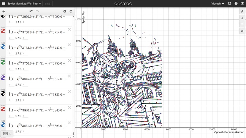
Spiderman
-
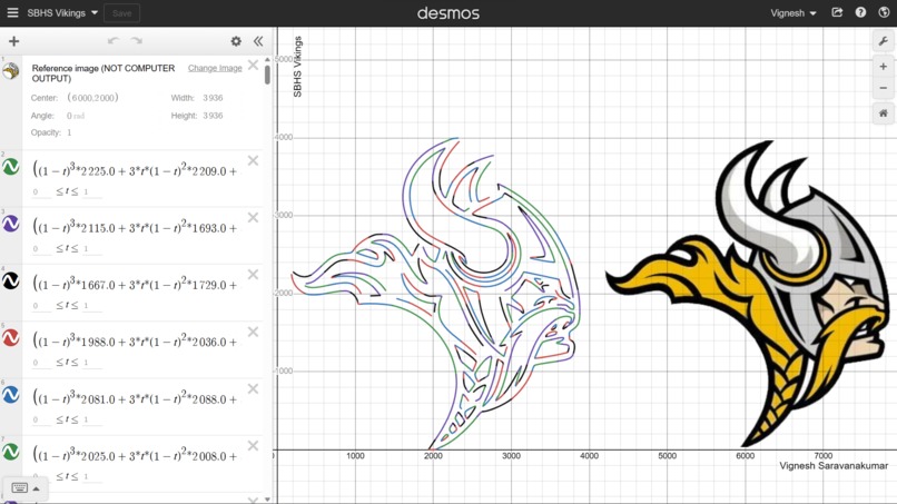
Viking
-
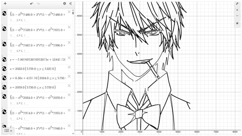
Manga
-
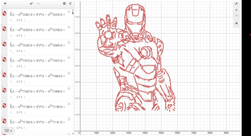
Iron Man


Inspiration
When learning about SVG file formats for an Android development class, mobile apps commonly use this format, I came to realize that SVG files held a unique property. Unlike other file formats, SVG files use mathematical equations to store an image instead. These equations would then be graphed by a computer. As someone who also liked playing around with mathematical equations on desmos, a graphing tool, I wanted to make use of this unique file format to display images on desmos using equations.
What it does
This program converts an image into a set of graphable equations. These are then graphed on demos using its API. This program takes advantage of a file format called SVG (Scalable Vector Graphics). Unlike other methods of encoding images, like PNG and JPEG, SVG files encode the image using mathematical equations. For this reason, SVG files are very compact and often used in 2D website design. Even Android Studio makes use of it for storing icons. Below is an example of an SVG file that represents Python's logo:<?xml version="1.0" standalone="no"?>
<!DOCTYPE svg PUBLIC "-//W3C//DTD SVG 20010904//EN"
"http://www.w3.org/TR/2001/REC-SVG-20010904/DTD/svg10.dtd">
<svg version="1.0" xmlns="http://www.w3.org/2000/svg"
width="2000.000000pt" height="1270.000000pt" viewBox="0 0 2000.000000 1270.000000"
preserveAspectRatio="xMidYMid meet">
<svg width="24" height="24" viewBox="0 0 24 24" xmlns="http://www.w3.org/2000/svg">
<path d="m14.31.18.9.2.73.26.59.3.45.32.34.34.25.34.16.33.1.3.04.26.02.2-.01.13V8.5l-.05.63-.13.55-.
21.46-.26.38-.3.31-.33.25-.35.19-.35.14-.33.1-.3.07-.26.04-.21.02H8.83l-.69.05-.59.14-.5.22-.41.27-.
33.32-.27.35-.2.36-.15.37-.1.35-.07.32-.04.27-.02.21v3.06H3.23l-.21-.03-.28-.07-.32-.12-.35-.18-.36-.
26-.36-.36-.35-.46-.32-.59-.28-.73-.21-.88-.14-1.05L0 11.97l.06-1.22.16-1.04.24-.87.32-.71.36-.57.4-.
44.42-.33.42-.24.4-.16.36-.1.32-.05.24-.01h.16l.06.01h8.16v-.83H6.24l-.01-2.75-.02-.37.05-.34.11-.31.17
-.28.25-.26.31-.23.38-.2.44-.18.51-.15.58-.12.64-.1.71-.06.77-.04.84-.02 1.27.05 1.07.13zm-6.3 1.98-.23.
33-.08.41.08.41.23.34.33.22.41.09.41-.09.33-.22.23-.34.08-.41-.08-.41-.23-.33-.33-.22-.41-.09-.41.09-.33
.22zM21.1 6.11l.28.06.32.12.35.18.36.27.36.35.35.47.32.59.28.73.21.88.14 1.04.05 1.23-.06 1.23-.16 1.04-.
24.86-.32.71-.36.57-.4.45-.42.33-.42.24-.4.16-.36.09-.32.05-.24.02-.16-.01h-8.22v.82h5.84l.01 2.76.02.36-
.05.34-.11.31-.17.29-.25.25-.31.24-.38.2-.44.17-.51.15-.58.13-.64.09-.71.07-.77.04-.84.01-1.27-.04-1.07-.
14-.9-.2-.73-.25-.59-.3-.45-.33-.34-.34-.25-.34-.16-.33-.1-.3-.04-.25-.02-.2.01-.13v-5.34l.05-.64.13-.54.
21-.46.26-.38.3-.32.33-.24.35-.2.35-.14.33-.1.3-.06.26-.04.21-.02.13-.01h5.84l.69-.05.59-.14.5-.21.41-.28.
33-.32.27-.35.2-.36.15-.36.1-.35.07-.32.04-.28.02-.21V6.07h2.09l.14.01.21.03zm-6.47 14.25-.23.33-.08.41.08.
41.23.33.33.23.41.08.41-.08.33-.23.23-.33.08-.41-.08-.41-.23-.33-.33-.23-.41-.08-.41.08-.33.23z"/>
</svg>

Given distinct points $P_{0}$ and $P_{1}$, a linear Bézier curve is simply a line between those two points. The curve is given by: ${\displaystyle \mathbf {B} (t)=\mathbf {P} _{0}+t(\mathbf {P} _{1}-\mathbf {P} _{0})=(1-t)\mathbf {P} _{0}+t\mathbf {P} _{1},\ 0\leq t\leq 1}$ Given distinct points $P_{0}$, $P_{1}$, and $P_{2}$, a quadratic Bézier curve is: ${\displaystyle \mathbf {B} (t)=(1-t)[(1-t)\mathbf {P} _{0}+t\mathbf {P} _{1}] +t[(1-t)\mathbf {P} _{1}+t\mathbf {P} _{2}],\ 0\leq t\leq 1}$ Given distict points $P_{0}$, $P_{1}$, $P_{2}$, and $P_{3}$, a cubic Bézier curve is: ${\displaystyle \mathbf {B} (t)=(1-t)^{3}\mathbf {P} _{0}+3(1-t)^{2}t\mathbf {P} _{1}+3(1-t)t^{2}\mathbf {P} _ {2}+t^{3}\mathbf {P} _{3},\ 0\leq t\leq 1.}$ Once the equations are placed in this parametric form, the equations can be placed in desmos to be graphed. Since desmos' API relies on your local browser to render the graphs. An HTML desmos graph is constructed using desmos API. The HTML file is then opened by the browser.
How we built it
The app was built using Python and desmos. Documentation for SVG files was consulted. In addition, Wikipedia and my math textbook were used to understand the math behind the bezier curves.
Challenges we ran into
One of the main challenges I ran into was understanding the math and the formatting of an SVG file. The varying formats used made it quite difficult to make the project work for all SVG file formats. In addition, the conversion of the bezier curves posed a challenge due to the mathematical complexity of converting bezier points to parametric equations. I overcame the SVG file formatting problems by using regular expressions instead of XML parsing libraries to extract the paths. The mathematical aspect was made simpler by revisiting an old calculus textbook.
Accomplishments that we're proud of
I am personally proud of the fact that I didn't give up on problems I encountered. I had several first attempts where the graphs looked like this: https://www.desmos.com/calculator/pnxiljwbbb. I had almost no idea how to fix things and had to resort to manually computing some of the curves in order to test the program.
What we learned
Through this I gained a deeper understanding of calculus, finding some real-life applications of it instead of simply learning from a textbook. In addition to this, I also managed to explore new libraries in Python and improve my programming skills.
What's Next for Image to Equations
In the future, I can learn to incorporate more complex curves like quartic and arc bezier curves. Attempts can also be made to animate the curves. Also, attempts can be made to represent entire videos as mathematical equations. This would mean videos can be played in a graphing utility like desmos.
Built With
- desmos
- python


Log in or sign up for Devpost to join the conversation.