Hydro Sentinel

Inspiration

Most water quality monitoring depends on physical sensors, but these sensors are expensive, limited, and absent from many rivers and lakes that need monitoring. The Ravi River runs through my city, Lahore, yet there is no continuous water quality monitoring along it. At the same time, satellites pass over the river every few days and provide multispectral imagery for free. That gap between available satellite data and places without monitoring inspired HydroSentinel. I was also interested in a common machine learning problem: a model can perform well when training and testing locations overlap but fail on completely new locations. I wanted to test HydroSentinel against this problem instead of relying only on a random train and test split.

What It Does

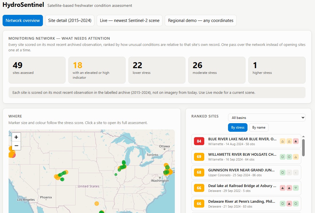
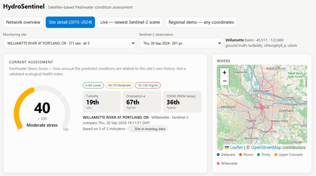
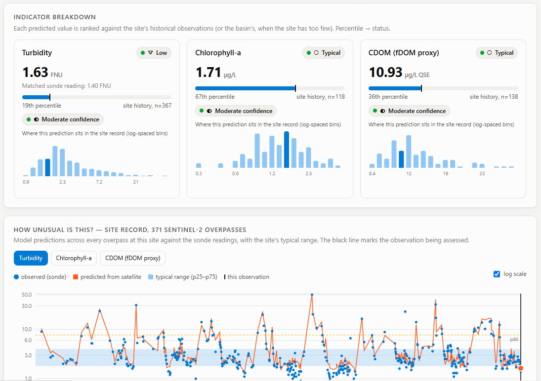
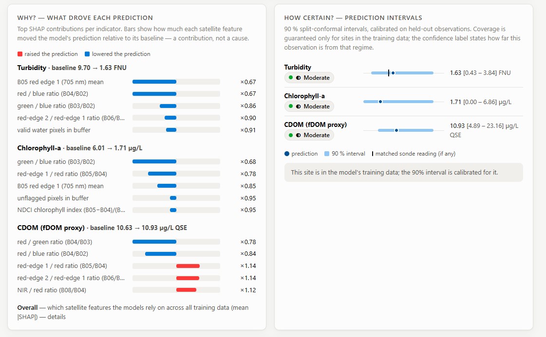
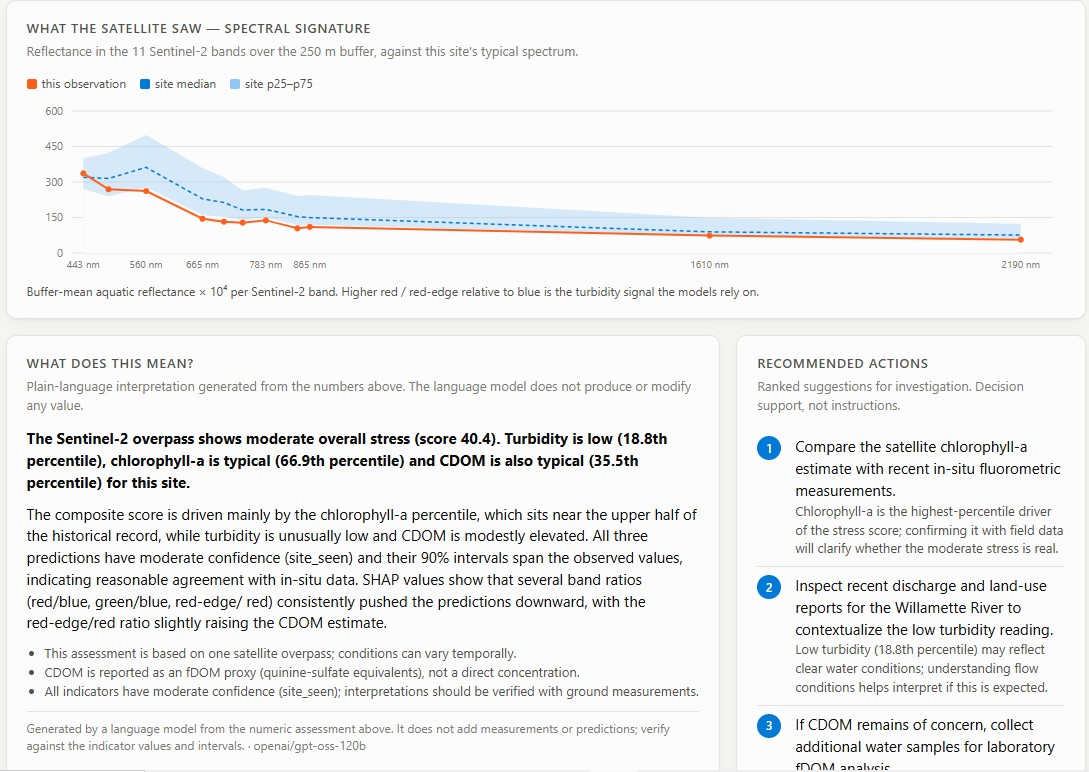
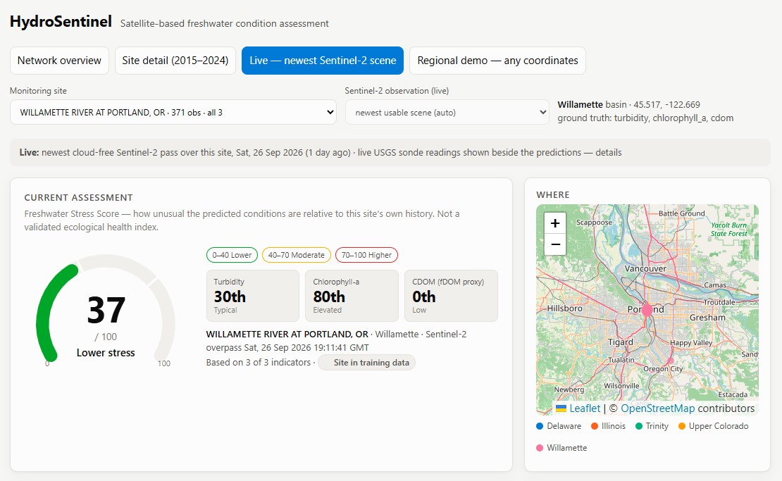
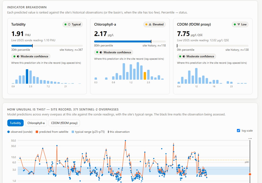
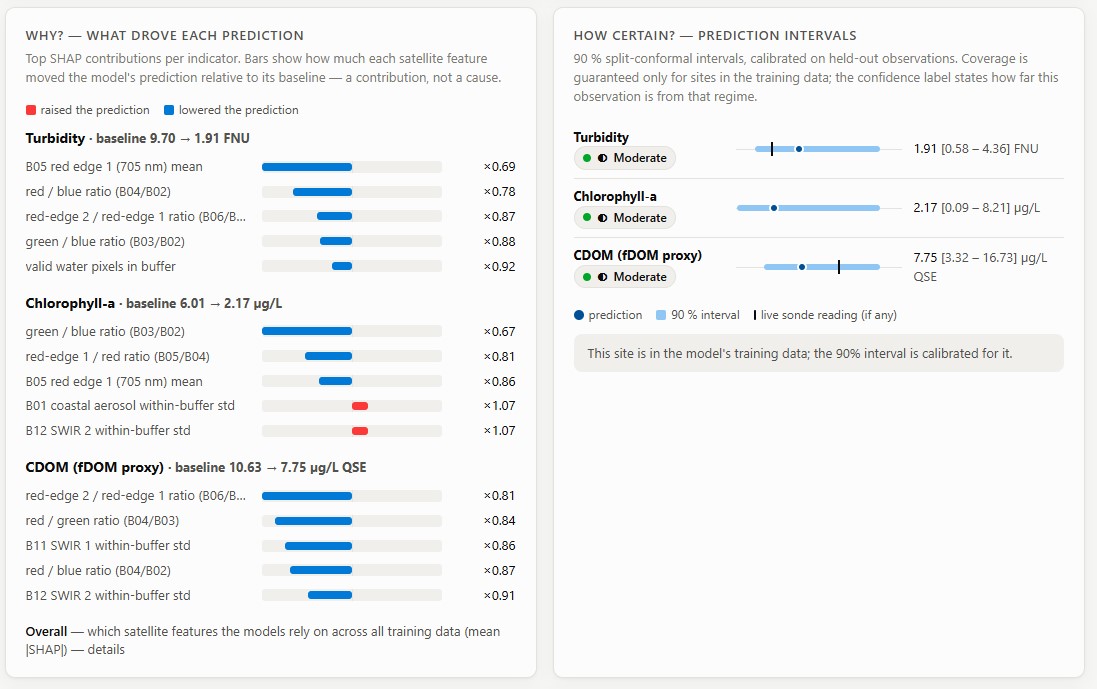
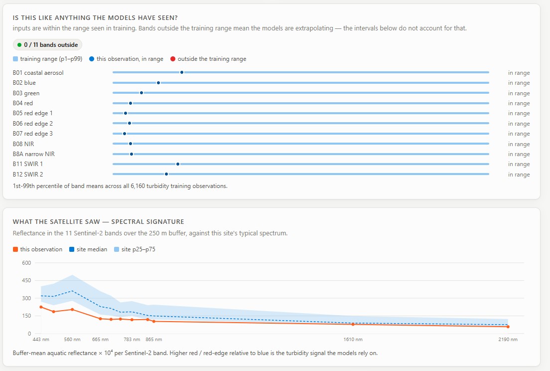
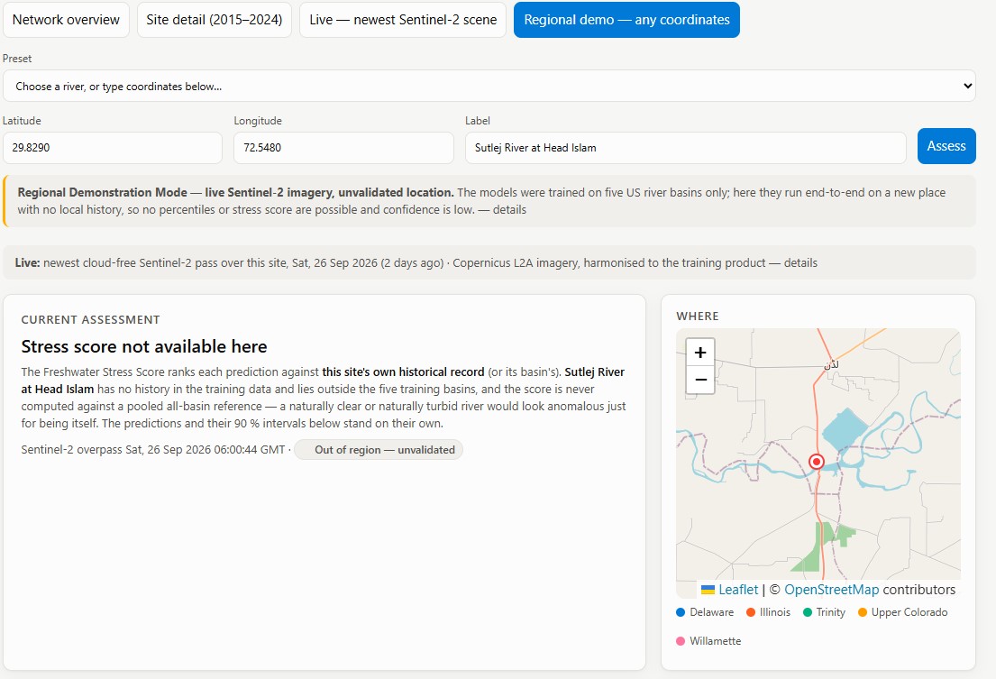
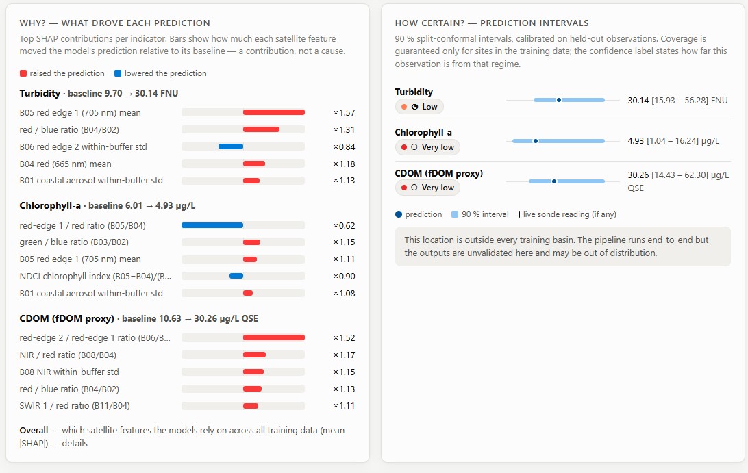
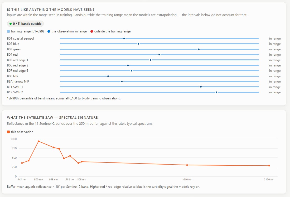
HydroSentinel estimates turbidity, chlorophyll a, and CDOM in rivers and lakes using Sentinel 2 satellite reflectance. For each estimate, it measures how unusual the current reading is compared with the historical behavior of that location, explains the prediction using SHAP, and provides a calibrated uncertainty interval using conformal prediction. The dashboard includes network, site, live, and regional views. It can rank monitored locations by current stress, provide detailed assessments, compare satellite estimates with real sensor readings, and score locations around the world, including places with no training data such as the Ravi River in Lahore. HydroSentinel does not forecast future conditions. It focuses on a different question: what is happening in the water right now, how unusual is it, and how confident are we in the estimate?

How I Built It

The training data came from a USGS dataset pairing Sentinel 2 aquatic reflectance with water quality measurements across five US river basins from 2015 to 2024. I compared XGBoost, LSTM, FT Transformer, and stacked models using site holdout and leave one basin out testing. XGBoost became the final model. LSTM was the closest alternative but required six previous observations from the same location, making it unsuitable for single observations and new locations. I used split conformal prediction in log space for uncertainty estimation and SHAP for model explanations. Stress scores are calculated against the location's own history whenever possible, with basin level fallback when local history is insufficient. For live US scoring, the backend reads satellite data directly from the USGS aquatic reflectance product. Outside the US, it uses the public Copernicus Sentinel 2 archive. For locations without historical records, the system builds a local anomaly score from roughly two years of satellite observations and clearly labels it as a model generated result. The backend uses FastAPI and the frontend uses React. Trained models and processed data are included in the repository so the deployed application does not need to download the full 1.4 GB raw dataset.

Challenges I Faced

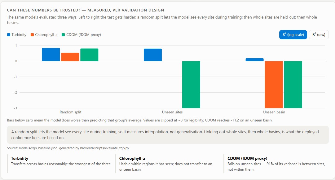
The biggest surprise was CDOM. It achieved an R squared value of around 0.69 on a random split, but when tested on an unseen basin, the R squared dropped to between negative 3 and negative 39. Around 91 percent of the variation came from differences between the six CDOM measurement sites rather than changes within individual sites. Instead of hiding this result, I kept CDOM as an experimental indicator and allowed the evaluation results to determine its confidence level. Another challenge was combining satellite data from different sources. The USGS training data uses ACOLITE while Copernicus uses Sen2Cor, which can produce different reflectance values for the same location. I compared 15 same day image pairs, measured the difference, and applied an adjustment before using Copernicus data outside the training region. The adjustment and its variation remain visible as part of the uncertainty. Security was also important. I identified an SSRF risk caused by external satellite URLs being passed directly to GDAL. I added an allowlist, addressed prompt injection through location labels, added rate limits to expensive endpoints, and introduced cache size limits with test coverage.

What I Learned

Random train and test splits are not enough for geospatial machine learning. A model can appear accurate when it has already seen the locations represented in the test data. Leave one basin out testing provides a clearer picture of how the model behaves in a genuinely different environment. I also learned that uncertainty should be part of the prediction itself, not something added later to the dashboard. Knowing where a model works, where it fails, and how confident it is is just as important as its overall metric.

What's Next

A newer USGS chlorophyll a dataset covering Oregon, Ohio, and Florida was released after the current pipeline was completed. Integrating it would provide more locations for testing generalization across different basins. The next major direction is forecasting. This would require its own data study because satellite revisit times, cloud cover, rainfall, river discharge, water levels, and longer time series all affect whether reliable forecasting is possible. I want to establish that the data can support forecasting before choosing a model, rather than adding predictions simply for the sake of having them.