-
Architecture
Clairvoyance by JAEGERS
Inspiration
House Edge asks for something most forecasting contests don't: the true probability of each payout, not the outcome. Every spin pays 0x, 1x, 2x, 5x or 20x, and we are scored on how close our five probabilities land to the simulator's hidden ones. A lucky jackpot doesn't help; only a calibrated forecast does.
That framing made it a puzzle about hidden structure. The rules say outcomes interact at lags of up to eight ticks, machines of the same type can react in opposite directions, and some episodes drift or change all at once. We wanted to find out how much of that structure could be recovered from history alone, without fooling ourselves with a validation set we had already looked at.
The scoring rule
For query \(i\) with forecast \(\hat{\mathbf{p}}_i\) and the simulator's true distribution \(\mathbf{p}_i\) over payouts \(s \in \{0, 1, 2, 5, 20\}\), the error averages over the 8 machines in an episode, then over the episodes \(\mathcal{E}_c\) in each condition \(c\):
$$ E_c = \frac{1}{|\mathcal{E}_c|} \sum_{e \in \mathcal{E}_c} \frac{1}{8} \sum_{i \in e} \left\lVert \hat{\mathbf{p}}_i - \mathbf{p}_i \right\rVert_2^2 $$
\(B_c\) is the same error for the organizers' frozen starter model. The four conditions (stable, short history, drift, shared change) count equally:
$$ R = \frac{1}{4} \sum_{c} \frac{E_c}{\max(B_c,\ 10^{-9})}, \qquad \text{points} = \frac{P_{\max}}{1 + R} $$
Matching the starter gives \(R = 1\), half the points; a perfect forecast gives \(R = 0\). Our local kit checkers report the main round out of \(P_{\max} = 60\) and the adaptation round out of \(P_{\max} = 20\).
What it does
Our submitted model, the Structural Stack, forecasts five payout probabilities for every query in both rounds and beats our own earlier champion on public validation in both. It runs fully offline in about 30 to 70 seconds on 2 CPU cores, refitting everything from the round's training split.
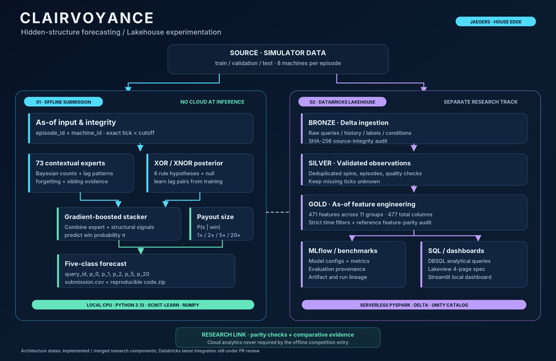
Every forecast factors into a win probability and a payout size given a win:
$$ \hat{p}(0) = 1 - \hat{\pi}, \qquad \hat{p}(s) = \hat{\pi} \cdot \hat{q}(s), \quad s \in \{1, 2, 5, 20\}, \qquad \sum_{s} \hat{q}(s) = 1 $$
The model has three layers:
- 73 lag-context experts (our original champion) estimate \(\hat{\pi}\) from each machine's own history, with evidence borrowed from the other machines in the same episode.
- A structural rule posterior tracks, online, which of six XNOR/XOR rules over win/loss at three lag pairs a machine is following, plus a no-rule null.
- A gradient-boosted stacker (scikit-learn HistGradientBoosting) combines both into the final \(\hat{\pi}\). Separate payout-size experts produce \(\hat{q}(s)\).
| Round | Our champion | Structural Stack | Starter baseline |
|---|---|---|---|
| Main (validation, kit checker, out of 60) | 55.091 | 55.485 | 30.000 |
| Adaptation (validation, kit checker, out of 20) | 18.245 | 18.392 | 10.000 |
All scores are public validation on Linux, from the exact submitted code. They are development scores, not hidden test results.
How we built it
We built a strong champion first, then spent the rest of the event trying to beat it under strict rules, and most challengers failed. The champion went from 51.55 to 54.99 to 55.12 out of 60 on public validation in its first afternoon, as we added size experts, peer evidence from sibling machines and the stacker.
The champion: a mixture of lag-context experts
Let \(w_t = \mathbb{1}[y_t > 0]\) be whether the spin at tick \(t\) won. Expert \(e\) looks at a context \(x_{e,t}\) built from one or two lagged outcomes (for example \((w_{t-2}, w_{t-5})\)) and keeps exponentially forgotten counts of wins \(W_e\) and visits \(N_e\) per context value. It predicts with a prior centred on the machine's recent win rate \(\bar{w}\):
$$ p_{e,t} = \frac{W_e(x_{e,t}) + \kappa\, \bar{w}}{N_e(x_{e,t}) + \kappa} $$
Each expert's forgotten log-likelihood on the machine's own past is
$$ \ell_{e,t} = \lambda\, \ell_{e,t-1} + w_t \log p_{e,t} + (1 - w_t) \log(1 - p_{e,t}), $$
and the experts are mixed by a softmax that also rewards experts that predict well on sibling machines in the same episode (\(\bar{\ell}^{\,\text{sib}}_e\)), plus a prior learned from the round's training machines:
$$ \alpha_e \propto \exp\!\left(\beta \left(\ell_e + \omega\, \bar{\ell}^{\,\text{sib}}_e\right) + \gamma \log \rho_e\right), \qquad p^{\text{mix}} = \sum_e \alpha_e\, p_e $$
The stacker then maps a feature vector \(\mathbf{z}\) describing the blend (mixture, top and second expert, top weight, disagreement, machine type, and so on) to the final win probability, \(\hat{\pi} = \sigma\!\left(f_{\text{HGB}}(\mathbf{z})\right)\). It is trained on historical ticks, with features computed only from ticks before each one.
Team and workflow
We ran the project like an engineering team, with AI coding agents (Codex/ChatGPT, Claude Code, Google Antigravity, Grok and Cursor) as teammates. Each agent claimed one GitHub issue, worked on its own branch and worktree, and opened a pull request that a human reviewed and merged. An automated check blocked PRs without a valid claim or that overlapped another open PR.
Research infrastructure on Databricks
We used Databricks to build a reproducible research infrastructure for probabilistic forecasting, rather than simply using it as a cloud training environment.
Our Serverless PySpark and Delta Lake Medallion pipeline ingests raw simulation data, validates historical observations, and produces 471 engineered forecasting features. We integrated Unity Catalog for data organization, feature-parity auditing for consistency, MLflow for experiment provenance, and SQL analytics for model comparisons and monitoring.
Our distinctive focus was scientific reproducibility: tracking exactly which data, features, models, and evaluation procedures produced each result, while separating training-based evidence from public-validation results. The final forecasting model runs independently offline; Databricks supports the research and analysis surrounding it.
Guardrails against fooling ourselves
- Pre-registration: each experiment's hypotheses and pass rule were committed before any result was computed.
- Two evaluations: the official validation score, plus a registry of 4 episode-grouped folds on the training split that never touches validation answers.
- Paired episode bootstrap: every comparison reports a 95% interval over whole episodes, not just a point score.
- Leakage audits: we tested that predictions never change when future ticks are added or removed, and that a missing tick stays unknown instead of becoming a loss.
The paired bootstrap resamples whole episodes within each condition, \(b = 1, \dots, 5000\), and recomputes both models' points on the same resample:
$$ \Delta^{(b)} = \text{points}_{\text{new}}^{(b)} - \text{points}_{\text{champion}}^{(b)}, \qquad \text{CI}_{95\%} = \left[\Delta_{(2.5\%)},\ \Delta_{(97.5\%)}\right] $$
What we tried, and what happened
Official validation points out of 60; champion 55.12.
| Challenger | Idea | Result |
|---|---|---|
| Dirichlet, Markov and decay models | Classical Bayesian count models | Best 43.98; not promoted |
| HMM, AR(1) and factorized regime models | Hidden-state temporal models | Best 46.18; not promoted |
| Champion + factorized blend | Linear ensemble | Optimal weight was 100% champion |
| Learned size regimes in the champion | Replace fixed payout-size constants | -1.05 points |
| As-of (causal) stacker | Remove train/serve skew in stacker rows | -0.29 to +0.01; only the free prior fix was neutral |
| 12 component ablations | Remove one part at a time | All worse or tied; the stacker alone is worth 2.29 |
| Structural Stack | Add rule-posterior features to the stacker | +0.39 [+0.03, +0.84]; promoted |
The negative results mattered: they told us the champion's lag experts already captured what generic time-series models could, so a gain had to come from the simulator's specific structure.
How we chose the Structural Stack
We chose it because it was the only challenger that beat the champion on two independent checks, and the reason it works is a structure we found in the simulator, not a tuned constant.
- Find the weakest condition. Short history was our worst condition (loss ratio 0.117 vs 0.067 to 0.092 for the others). Swapping in the true win probability cut it to 0.047, while swapping in the true payout sizes only cut it to 0.071. So the error was mostly whether a machine wins, not how much.
- Look for the simulator's rule. On training machines, the best expert was almost always one of three lag pairs, and the win rule was XNOR or XOR of win/loss at that pair. Six hypotheses covered 152 of 183 stable machines. With only about 64 observed ticks, the champion couldn't identify the rule; an explicit rule posterior can.
- Test it as pre-registered experiments. A stronger expert prior was neutral (-0.04). A standalone rule model was worse. Feeding four rule-posterior features into the existing stacker was the winner.
- Confirm on data validation never touched. A walk-forward test on the training split (40 earlier cutoffs per held-out episode, 30,720 labels) improved Brier by 0.0034 [0.0027, 0.0041], with short history improving most. Validation agreed: +0.39 points [+0.03, +0.84], short-history loss ratio 0.117 to 0.089.
- Make it reproducible. Windows and Linux outputs differed beyond the \(10^{-8}\) reproduction tolerance, so we pinned NumPy and OpenBLAS CPU dispatch and generated the submission on Linux. Two cold runs from the ZIP gave byte-identical CSVs.
- Adapt it for round two. The adaptation simulator changed the lag pairs. We made the model learn its pairs from the round's training histories (no labels, no validation). That raised it from a tie with the champion (18.257 vs 18.245) to 18.392, a gain of +0.146 [+0.021, +0.282] in a paired episode bootstrap.
The rule hypotheses
For a lag pair \((a, b)\), the rule is "on" when the two lagged outcomes agree (XNOR) or disagree (XOR):
$$ r^{\text{XNOR}}_{a,b}(t) = \mathbb{1}\!\left[w_{t-a} = w_{t-b}\right], \qquad r^{\text{XOR}}_{a,b}(t) = 1 - r^{\text{XNOR}}_{a,b}(t) $$
Hypothesis \(k\) predicts a high win rate when its rule is on and a low one when it is off, with \(p_{\text{on}}\) and \(p_{\text{off}}\) pooled across training machines. The null hypothesis \(k = 0\) predicts the machine's own forgotten win rate \(\bar{w}_t\):
$$ P_k(w_t = 1) = \begin{cases} p_{\text{on}} & r_k(t) = 1 \\ p_{\text{off}} & r_k(t) = 0 \end{cases}, \qquad P_0(w_t = 1) = \bar{w}_t $$
If either lagged tick is missing, the hypothesis abstains and falls back to \(\bar{w}_t\). A missing tick is never treated as a loss.
The online posterior
Each hypothesis accumulates a forgotten log-likelihood over the machine's observed ticks before the cutoff \(c\), and a prior \(\pi^{(0)}_k\) counts how often \(k\) was the best rule on training machines:
$$ L_k(t) = \lambda L_k(t-1) + \log P_k(w_t), \qquad \pi_k(c) = \frac{\pi^{(0)}_k\, e^{L_k(c)}}{\sum_j \pi^{(0)}_j\, e^{L_j(c)}} $$
$$ \pi^{\text{rule}}(c) = \sum_{k=0}^{6} \pi_k(c)\, P_k(w_c = 1) $$
The forgetting rate \(\lambda \in \{1, 0.99, 0.97\}\) is chosen on training labels.
Four new stacker features
The stacker gets four extra inputs, all computed only from ticks before the row's tick:
$$ \mathbf{z}^{\text{rule}} = \Big(\operatorname{logit} \pi^{\text{rule}},\ \max_{k \ge 1} \pi_k,\ \pi_0,\ \operatorname{logit} \pi^{\text{rule}} \cdot \max_{k \ge 1} \pi_k\Big) $$
The idea: when the posterior is confident, the stacker can trust the rule's prediction even with few observations. When the null wins, it falls back on the lag experts.
Learning the lag pairs (adaptation)
Our main-round version hard-coded the pairs \((1,3), (2,5), (4,7)\). In the adaptation kit those stopped working. For every training machine \(m\) and every pair \(1 \le a < b \le 8\), we measure how well the best rule at that pair fits its observed history:
$$ \text{acc}_m(a, b) = \max\big(\text{agree}_m(a, b),\ 1 - \text{agree}_m(a, b)\big), \qquad \text{agree}_m(a, b) = \frac{1}{|T_m|} \sum_{t \in T_m} \mathbb{1}\!\left[r^{\text{XNOR}}_{a,b}(t) = w_t\right] $$
Here \(T_m\) is the set of ticks where \(w_t\), \(w_{t-a}\) and \(w_{t-b}\) are all observed, with at least 30 required. Each machine votes for its best pair, and we keep the three pairs with the most votes:
$$ \mathcal{P} = \operatorname{top}_3 \sum_{m} \mathbb{1}\!\left[(a, b) = \arg\max_{(a', b')} \text{acc}_m(a', b')\right] $$
| Training split | Top 3 pairs (\(\mathcal{P}\)) | Share of machines |
|---|---|---|
| Main | (4,7), (2,5), (1,3) | 26.0%, 25.4%, 23.6% |
| Adaptation | (3,8), (1,4), (2,6) | 24.7%, 23.6%, 19.8% |
On main data it recovers exactly the pairs we had hard-coded; on adaptation data it finds the new ones. It uses no labels and no validation data.
The trade-off we accepted
Drift is slightly worse than the champion in both rounds (adaptation loss ratio 0.103 vs 0.081). The gains in stable and short history are larger and consistent across episodes: on adaptation validation, the Structural Stack beats the champion on 88% of stable episodes and 71% of short-history episodes.
Challenges we ran into
- Short histories. With 40 recent ticks and 24 scattered older ones, most lag contexts are seen only a handful of times. This was our worst condition all event and the main target of the final model.
- A validation set we had already looked at. Some champion settings were read off public validation answers, so its validation score flatters it. We added a second evaluation on training folds and a walk-forward test so no decision rested on validation alone.
- Subtle look-ahead. Our audit found three places where the stacker's historical training rows used information from after the row's tick, such as the query-time signal copied onto every past row. None leaked test labels, but fixing all three cost about 0.3 points, so we documented them and flagged them for organizer clarification rather than silently changing the champion.
- Byte-level reproducibility. The same code gave different probabilities on Windows and Linux, on 1,296 of 1,536 test queries. We pinned CPU instruction sets and thread counts and always generated the uploaded CSV on Linux.
- The pattern change in round two. Our main-round rule features were hard-coded to the main simulator's lag pairs and became useless when the adaptation kit changed them. We found this within minutes by scanning training histories, and fixed it inside the 90-minute window.
- Coordinating five AI agents. Parallel agents duplicated work and collided on files early on. Issue claims, one worktree per agent and an automated PR checker solved it.
Accomplishments that we're proud of
- Finding the simulator's rule. Recognizing that wins follow XNOR/XOR of two lagged outcomes turned a black box into a model with a mechanism, and it carried over to round two once the pairs were learned.
- Beating a strong baseline honestly. Our champion already scored over 55/60; the Structural Stack beat it in both rounds, with confidence intervals that exclude zero and a walk-forward check that never saw validation answers.
- Publishing negative results. More than a dozen pre-registered challengers and ablations didn't beat the champion, and we kept every one of them in the repo with its numbers.
- Reproducible submissions. Each upload is a CSV plus a code ZIP that regenerates it byte for byte from one command on Linux.
- A working multi-agent engineering process: claimed issues, isolated branches, reviewed pull requests and CI, with humans making every merge and submission decision.
What we learned
- Diagnose before you model. Substituting true quantities into our own forecast showed exactly where the error was. That one check pointed us at win probability in short histories and saved hours of tuning the wrong part.
- Mechanism beats model family. HMMs, Markov chains and blends all lost to the champion. A small feature encoding the simulator's actual rule won.
- Learn structure from data, don't hard-code it. The main-round lag pairs were right for main and useless for adaptation. Learning them from training histories cost nothing and made the model robust to the change.
- A score you've looked at is not evidence. Pre-registration, grouped folds and paired bootstraps let us separate real gains from noise; several "improvements" turned out to be inside the noise.
- Reproducibility is a feature you have to build. Floating-point differences between machines are real, and only pinning the environment made our ZIP reproduce our CSV exactly.
What's next
- Fix drift. It is the one condition where the Structural Stack is worse than the champion. A rule posterior that forgets faster, or one that tracks a rule reversing over time, is the obvious next experiment.
- Learn payout sizes per round. Our payout-size constants came from main-round data and may be off in a round where sizes change.
Built with
Python 3.13 · NumPy · SciPy · scikit-learn (HistGradientBoosting) · pytest · GitHub Issues, Pull Requests and Actions · WSL2 Ubuntu for Linux reproduction · uv · Databricks (Serverless PySpark, Delta Lake, Unity Catalog, MLflow, Databricks SQL) · Streamlit dashboard · AI coding agents: ChatGPT/Codex, Claude Code, Google Antigravity, Grok and Cursor
Built With
- bayesian-inference
- chatgpt
- claude-code
- cursor
- databricks
- delta-lake
- github
- github-actions
- google-antigravity
- gradient-boosting
- grok
- mixture-of-experts
- mlflow
- numpy
- probabilistic-forecasting
- pyspark
- pytest
- python
- scikit-learn
- scipy
- statistics
- streamlit
- time-series
- wsl2
