Hazard Vulnerability and Jurisdictional Risk Prediction Modeling of Ebola in West Africa Marcia A. Testa, MPH, PhD, Maxwell Su, ScD, Souley Konate, PhD, Jesus Torres and Elena Savoia, MPH, MD Department of Biostatistics Preparedness and Emergency Response Learning Center Division of Policy Translation and Leadership Development
Abstract:
Questions Asked: One of the major responsibilities of public health authorities is to identify population groups vulnerable to potential hazards including both natural and human-made hazards that could negatively impact the lives, economy, environment and property of residents living within the jurisdictions they serve. We evaluated the usefulness of employing population-averaged Poisson regression to inform a comprehensive Hazard Vulnerability and Jurisdictional Risk (HVJR) model (HVJR) in efforts to gain insight on preparedness planning and response to Ebola in West Africa. Data wrangled/processed: We used an HVJR model to conceptualize the vulnerability and resilience components and the outcomes of the Ebola hazard. We analyzed data provided by WHO and Ministries of Health on the reported number of cases and deaths. We evaluated the vulnerability indicators from the dataset entitled “Subnational Indicators Ebola Countries”. We also used regional population size and population density data. Data were merged into a relational database yielding 34 regions and serially time points of cases and vulnerability covariates.
Analysis Approach: We utilized ArcGIS (ArcMap) to visualize the epidemic, health resources and structural environment of the West African countries affected by Ebola. We employed a longitudinal, population-averaged Poisson model (xtpoisson command in Stata 13.0) and epidemic growth curves for prediction. For the Poisson model, we used “Region” as the sampling unit and “population size” as the Poisson “exposure” variable. The data were first set using the Stata command “xtset sdr_id dates” to declare the regions (i.e., sdr_id variables) as the “subject” variable and the dates of each case report (converted to weekly intervals) as the “repeated measures” variable. We divided the data into two data sets “Pre October 1, 2014” with 359 rows “Full Period” (through November 16, 2014) with 522 rows.
Preliminary Findings: First, not controlling for any vulnerability indicators, for the period up through October 1, 2014, as compared to Sierra Leone Guinea had a 77% lower incidence rate ratio (IRR – from Poisson model) an Ebola case while Liberia had a 51% higher IRR. Of the vulnerability indicators, percent of children less than 9 years (p =0.000), urban areas (p = 0.032), and percent of households with electricity (p =0.020) were all protective indicators. These covariates explained a substantial amount of the risk difference between Liberia and Sierra Leone. Using the predicted cases as a base rate and under an epidemic weekly 0.06 growth parameter (from epidemic model), we predicted that an additional 3,660 cases would occur over the remaining 7-week interval, when in fact 3,667 cases occurred. The model that included all data through November 16, 2014 showed that the IRR of the three countries were coming closer during the latter 7-week interval, especially for Liberia which as compared to Sierra Leone was no longer statistically significantly different (IRR = 1.09, P = 0.755) reflecting increasing risk in Sierra Leone. The differential between Sierra Leone and Guinea remained constant. After controlling for two vulnerability indicators, Guinea and Liberia had lower risk as compared to Liberia. Using this model and again a 0.06 weekly growth parameter an additional 4,148 cases are projected for the 7 weeks post November 16, 2014 through to the end of this year. However, changing infectivity rates, resilience and vulnerability need to be incorporated in these models for greater accuracy.
Future Planning: What is apparent for future 2015 forecasting is that the “Resilience” component of the HVJR model will most likely dominate “Vulnerability” factors. Since the resilience components are drastically improving, we caution against using the April, 2014 through November 15, 2014 to forecast January and February, 2015 cases and deaths simply based upon standard infectious disease modeling, but rather consider a more comprehensive hazard vulnerability and jurisdictional risk assessment model for public health emergency preparedness planning.
INTRODUCTION
One of the major responsibilities of public health departments is to identify population groups vulnerable to potential hazards including both natural and human-made hazards that could negatively impact the lives, economy, environment and property of residents living within the jurisdictions they serve. To carry out this function, town, city, county, prefecture and regional public health authorities must increasingly conduct hazard vulnerability and jurisdictional risk (HVJR) modeling as part of their public health emergency planning and response initiatives. While there are number of types of hazards that impact human, economic and structural losses, infectious diseases, such as Ebola, can be catastrophic if grass roots public health prevention measures such as case finding and tracking, use of personal protective equipment and quarantining the exposed and isolating the infected and are not initiated early and consistently.
Hazard Vulnerability and Jurisdictional Risk Assessment (HVJR) of Ebola: Conceptual Health Model
- Primary Question Asked: How can we use prediction regression modeling to identify potential (HVJR) “Vulnerabilities” in order to estimate the impact of increasing HVJR “Resilience” and reduction in mortality due to Ebola.
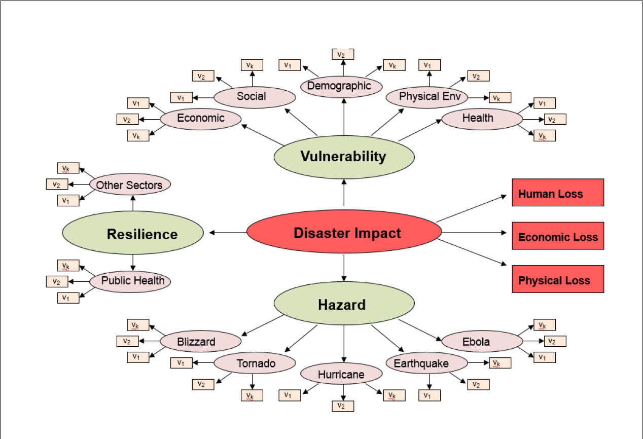
To formulate the analysis of the Ebola data, we first adopted the HVJR Conceptual Model to Ebola HVJR (1) (depicted in Figure 1 - Image Gallery) which we have utilized in our Preparedness and Emergency Response Learning Center at the Harvard School of Public Health. Here we consider only one hazard, Ebola, and only human losses (cases/deaths due to Ebola). The “Vulnerability” domain includes those socio-economic, demographic, health and physical environment factors (covariates) that make individuals more susceptible to exposure, infection and death. The “Resilience” factors include the governmental and public health infra structures that counter the negative impact of hazards and vulnerability. Our focus was to identify potential vulnerabilities in order to evaluate the impact of increasing “Resilience” for epidemic forecasting.
We first downloaded the sixteen *.csv files that were made available to the HackEbola (With Data) participants. We examined the data for accuracy and interpretability. We reviewed the data sources, structure and results of geospatial analyses and used ArcGIS - ArcMap to ascertain the regional variable definitions and to locate and examine the locations of the numbers of cases and deaths. Excerpted data rows from the case file is shown below.
Table 1. Example of Data File Number 2: Sub-national time series data on Ebola cases (Excerpted Rows) GN Guinea Conakry Cases 20 4/7/2014 WHO GN Guinea Conakry Deaths 6 4/7/2014 WHO GN Guinea Dabola Cases 4 4/7/2014 WHO GN Guinea Dabola Deaths 3 4/7/2014 WHO GN Guinea Dinguiraye Cases 1 4/7/2014 WHO GN Guinea Dinguiraye Deaths 1 4/7/2014 WHO GN Guinea Gueckedou Cases 90 4/7/2014 WHO GN Guinea Gueckedou Deaths 63 4/7/2014 WHO GN Guinea Kissidougou Cases 9 4/7/2014 WHO GN Guinea Kissidougou Deaths 6 4/7/2014 WHO GN Guinea Macenta Cases 27 4/7/2014 WHO GN Guinea Macenta Deaths 16 4/7/2014 WHO
Step 2: Geocoding search function (World Geocode Service)
We located each jurisdiction using the ArcGIS World Geocode Service. Selected excerpts for the country of Guinea are listed below.
- Dabola, Fanarah Region, Guinea
- Canokry, Canokry, Guinea
- Dinguiraye, Fanarah Region, Guinea
- Gueckedou, Nzerekore, Guineau
- Kissidougou, Fanarah Region, Guinea
- Macenta, Nzerekore, Guineau
- Nzerekore, Nzerekore, Guineau
Step 2: Ebola Cases from August 15, 2014 through October 15, 2014
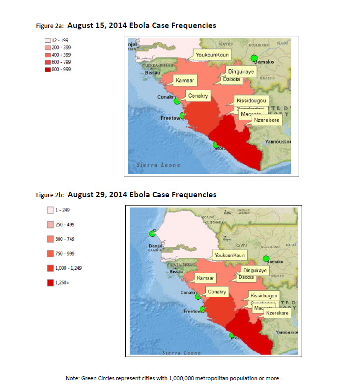
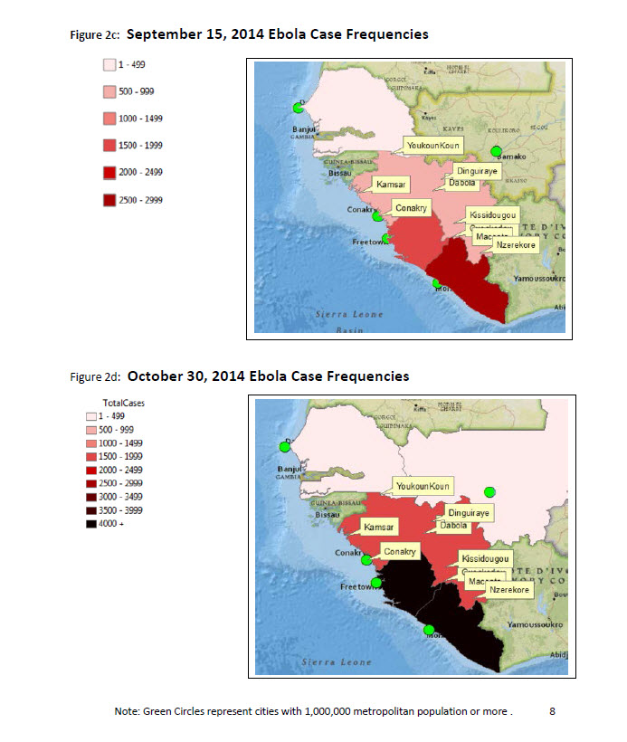
We then applied an Ebola (cases/deaths) layer using ArcMap to examine the August through end of October 2014 time-trends of the numbers of infected (cases) and associated deaths using data provided by ArcGIS Online Direct Relief Services data bases to compare with the data files downloaded from the Ebola Hackathon (With Data) Website. The graphical visualization results are shown in the four figures below (Figures 2a, 2b, 2c ad 2d - Image Gallery).
From this quick geospatial analysis, it was clear that the epidemic was primarily contained to the three primarily affected countries (Guinea, Liberia and Sierra Leone) and that the cases were increasing over time according to a fairly typical epidemic growth curve function, with an incubation period span of approximately 21 days peaking on average as follows for mild, moderate, severe symptoms and death.
Step 3: Creating the Analytical Dataset As a first step, we attempted to confirm which variables were appropriate, and where there might be duplicate responses. We first looked at the case/death file to determine the uniqueness of the region by date data points. We then examined the individual time curves by country to determine whether there were duplicate time points because of repeated data by the ‘Source’ variable and to get a better feel for the shape of the epidemic cumulative functions.
3) Analysis approach
Identifying the Regional “Sampling Units” and Covariates We originally identified 62 unique jurisdictional regions in the case file after eliminating the sdr-id = 0 values since these represented entire countries. We removed Mali, Senegal and Nigeria from further analyses. We collapsed the data to the Regional ADM1 levels and merged the data into one relational database containing the cases, population (exposure), dates and other “Vulnerability” covariates. This resulted in 34 ADM1 regional sampling units for purposes of modeling.
Epidemic Modeling versus Poisson Regression Methods
Initially we considered two different approaches to modeling.
- Stochastic Compartmental Models and Non-linear Regression
- Longitudinal Population-Averaged Poisson Regression
Since the populations of the affected countries were extremely large, the incidence of Ebola relatively rare, the cases and deaths had similar functions and the case fatality rate was high, we chose to use approach 2 to investigate the effects of the Vulnerability covariates on the probability of becoming infected. The initial random-effects, compartmental stochastic model considered initially, while intuitive attractive was not as amenable to regression and post-estimation contrasts for evaluating the vulnerability indicators.
4) Major findings, Implications and Limitations.
Longitudinal, population-averaged Poisson Regression Models
We employed a longitudinal, population-averaged Poisson model (xtpoisson command in Stata 13.0) for evaluating the expected number of cases and the impact of the Vulnerability indicators. We used the “Region” as the sampling unit of interest and the “population size” of that region as the Poisson “exposure” variable. The data were first set using command “xtset sdr_id dates” to declare the regions (i.e., sdr_id variable) as the “subject variable” and the “dates” of each case report (converted to weekly intervals to ensure relatively fewer non-missing cells) as the “repeated measures”. The “dates” variables were deemed time variables, however, we did not use a time-series or forecasting approach in this preliminary analysis. Future analyses will consider that option. We divided the data into two data sets “Pre September 30, 2014” with 359 rows of data and the October 1 - November 16, 2014 extended with 522 rows of data .
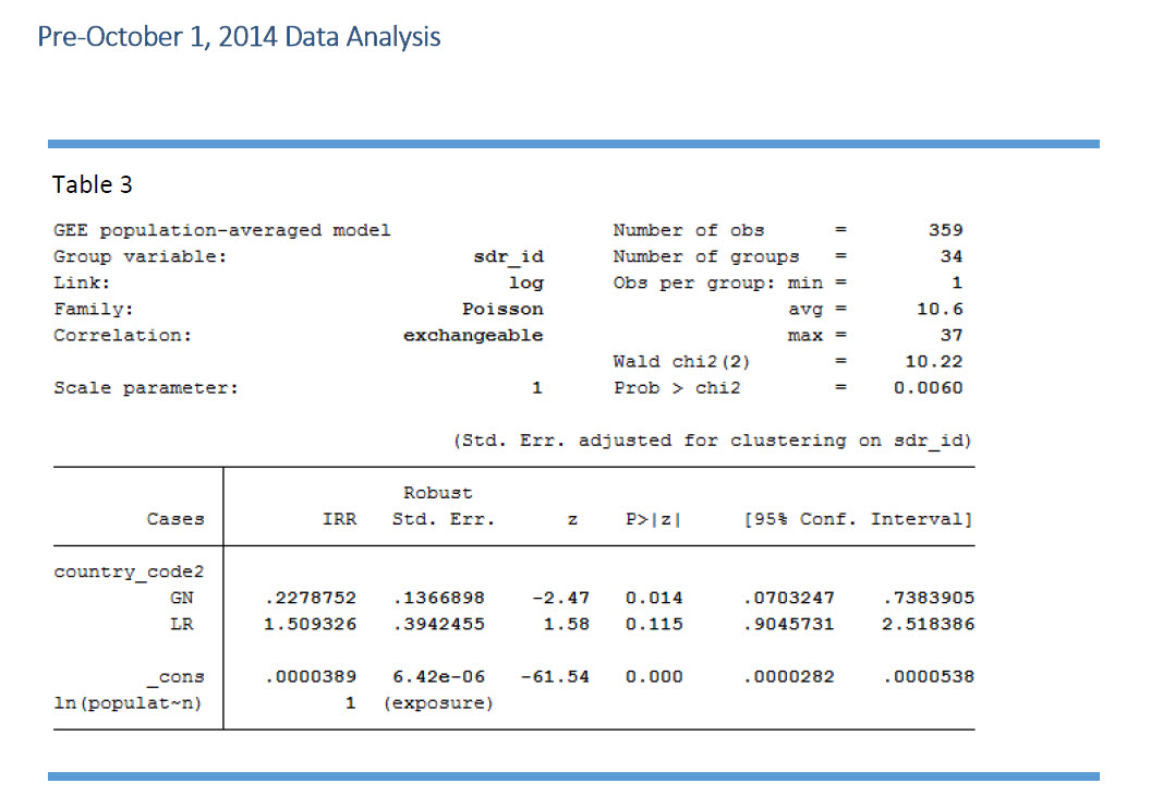
We began our modeling with a simplified crude Poisson regression model comparing the three affected countries without covariates. We report here the Incident Rate Ratios (IRRs) rather than the beta coefficients for interpretability. With this crude model, as compared to Sierra Leone, Guinea had approximately 77% lower IRR, not controlling for any covariates while Liberia had 51% greater IRR (See Table 3 - Image Gallery). We attempted to fit various fuller models with the set of covariates available, keeping in mind that we only had 34 “populations” to model and several highly correlated independent predictor variables.
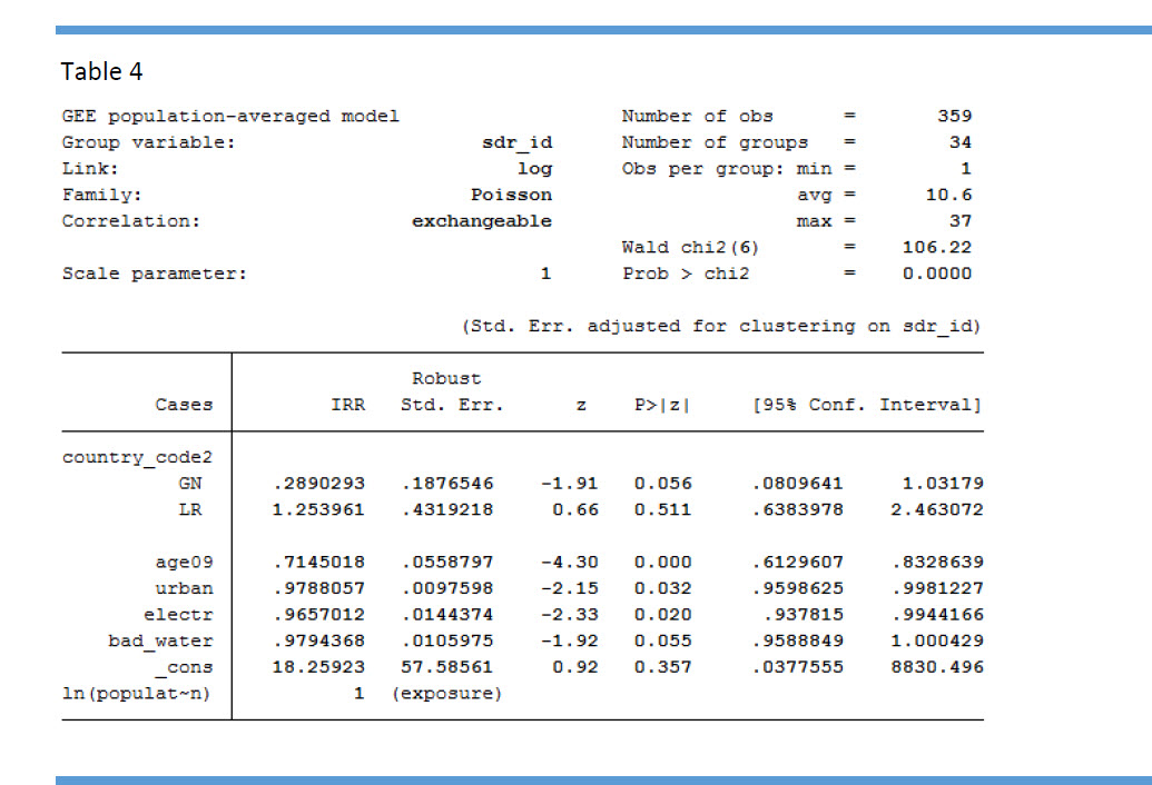
Subsequently, we fit a full model with the covariates listed in the Data Set “Subnational Indicators Ebola Countries” and we added the population “density” for each region as an additional variable. We noted that there was considerable collinearity among the covariates, and that the instability of the parameters estimates had to be evaluated cautiously. Ultimately, we reduced the parameters in the model as shown in Table 4 - See Image Gallery. Collectively, it appears that urban living, higher percentage of younger children and having electricity were all protective against risk. We again note that many of the independent variables were highly correlated and that those selected may be surrogates for a unifying domain of “higher socioeconomic status”. In addition, these vulnerability indicators help explain some of the variability between the countries as can be seen by the reduction in the differences in the IRRs associated with the “country effect” for the Liberia country effect.
Stata Command: xtpoisson Cases ib(last).country_code2 age09 urban electr bad_water , pa exposure(population) corr(exchangeable) vce (robust) irr
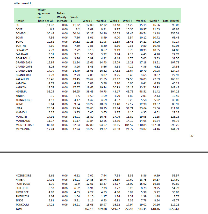
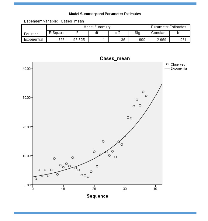
Predictions for Post-September 30, 2014 Period Based upon the estimated model given above, we determined the base rate predicted number of weekly cases for a given interval for each region. Using the post estimation command in Stata we calculated the base rate predicted number of cases per 7 day period. We calculated the time difference between September 30, 2014 and November 16, 2014 and multiplied this times the expected number of cases per week assuming an increasing rate of 6 percent weekly as estimated from the shape of the epidemic curves within each of the 34 regions. We determined the 6 percent increase ( b1 = 0.061 in Figure Epidemic Growth Parameter - See Image Gallery) per week examining the rate of increase from the epidemic growth curve using the same data set upon which the model was built. Summing over the 34 regions over the 7-week period we obtained a total expected increase in cases for that 7 week period of 3660 cases – (See Excel screenshot - Attachment 1 - Image Gallery).
Analysis through November 15, 2014 Analysis We first tested the validity or our Predicted Number of Cases Estimates using the Pre-October data by comparing it to the actual number of cases between October 1 and November 16, 2014. We note that the number of cases vary a bit from the daily totals because we used 7-day intervals. Using the 7-day interval data and the September 30, 2014 cutoff, we compared the observed number of cases across the three countries to the expected number of cases as shown below.
Predicted and Observed Number of Cases: 7 Weeks Post 9/30/2014 through 11/16/2014. Expected from Poisson/Epidemic Regression Model: 3,660 Observed Number of Cases: 3,667
Overall, the expected number of cases from the population-average Poisson Model for Pre-October was within 99.8% of the actual number occurring Post-October. We applied the increase in the hazard of infection from the epidemic curve. We also noted substantial variability among the observed and expected values across the 34 regions. By detecting early areas with much larger than expected cases for that interval and general region, it would be possible to target these areas for more intensive public health case finding and tracking, personal protective equipment (PPE) use, quarantine of the exposed and isolation of the infected.
Modeling the Full (Through November 16, 2014) Data Set
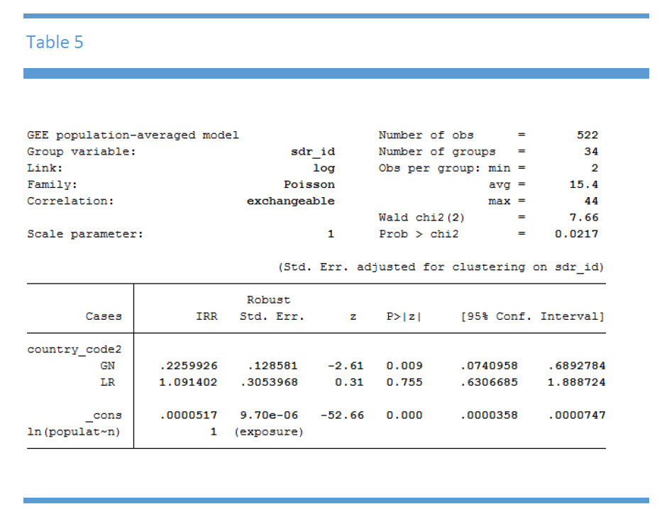
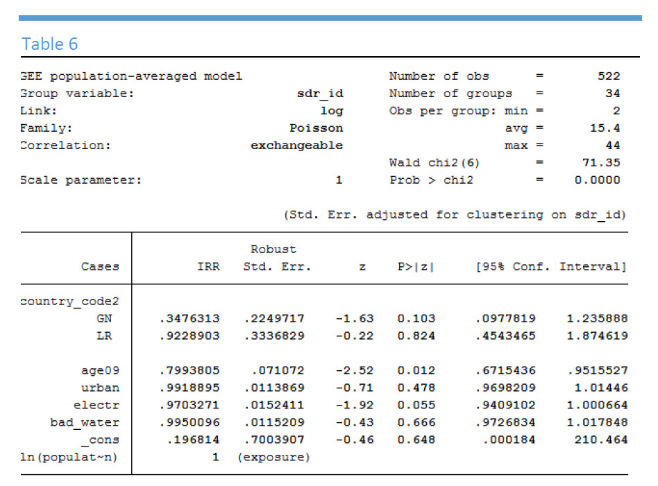
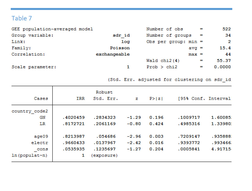
During the 6 weeks from the September 30 cutoff through November 16, 2014 the IRRs between Liberia and Sierra Leone became quite a bit closer (IRR = 1.09). (Table 5 - See Image Gallery) We ran several fuller covariate models including the final model for the Pre-October 1, 2014 data. For this final model, not all of the covariates that were statistically significant were significant for the more recent data (Table 6 - See Image Gallery). As such, we reduced the model further keeping in only “%younger children < 9 years” and “% of households with electricity” as indicators of vulnerability (Table 7 - See Image Gallery). The “electricity” variable is really a surrogate for high socioeconomic and urban status.
We then applied the prediction equation to project seven weeks forward from the November 16, through January 1, 2014 using the full data model. Again, we assumed that the hazard rate 6% during that period as was done previously by confirming the beta = 0.056 from the full data set. With the full data set, our estimate of the 7 week increase in cases for the next 7 week period was now 4,148 as compared to 3,660 from the earlier dataset. This beta increase assumption is again an oversimplification and assumes that the average case load will increase uniformly during the 7-week interval. In reality, the changing hazard coefficient should be a function of changes in both Resilience and Vulnerability and not just the epidemic growth curve. Under constant Resilience and Vulnerability assumptions, the change in the rate of infections per week will be a function of the natural history of the virus. When Resilience is increased as we expect it will be going forward the hazard will be reduced. If economic hardships continue, however, the Vulnerability will be increased as will the number of cases.
Summary Remarks and Looking Forward
Given the extraordinary Ebola containment efforts begun in October and November, 2014 it is unlikely that the Ebola epidemic will spread to surrounding countries in the same fashion as the initial April through October, 2014 outbreak. Moreover, if isolated cases do appear, current isolation and quarantine is being enforced and is extremely effective. This is already apparent for the countries of Senegal, Nigeria and Mali.
We conclude that the data from April through September, 2014 represented the first phase of the epidemic with high Vulnerability and low Resilience, and that the April through November, 2014 was fairly consistent with the typical epidemic curve function under those circumstances. What is apparent for the future 2015 forecasting is that the “Resilience” component of the HVJR model appears now to be dominant over “Vulnerability”. Increasing resilience serves as an intervention which will change the weekly growth increase in a downward fashion. While there is no data in the current data files to substantiate this, our perspective is based upon recent global efforts to assist in this outbreak. We anticpate that the Resilience components will be dominant moving forward into January 2015.
No longer are the local regions the only Resilience contributors, rather, local regional vulnerabilities now appear to be strongly outweighed by a strong global response.
Because the resilience components are steadily improving, we caution against using the April, 2014 through November 15, 2014 to forecast January and February, 2015 cases and deaths simply based upon standard infectious disease modeling. Rather we recommend considering a more comprehensive hazard vulnerability and jurisdictional risk assessment model for public health emergency preparedness planning.
References Testa MA, Pettigrew ML and Savoia E. Measurement, geospatial, and mechanistic models of Public Health Hazard Vulnerability and Jurisdictional Risk, Journal of Public Health Management and Practice, J Public Health Manag Pract. 2014 Sep-Oct;20 Suppl 5:S61-8.
Built With
- sas-9.4
- spss-22
- stata-13


Log in or sign up for Devpost to join the conversation.