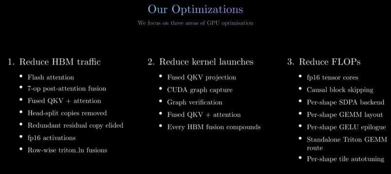
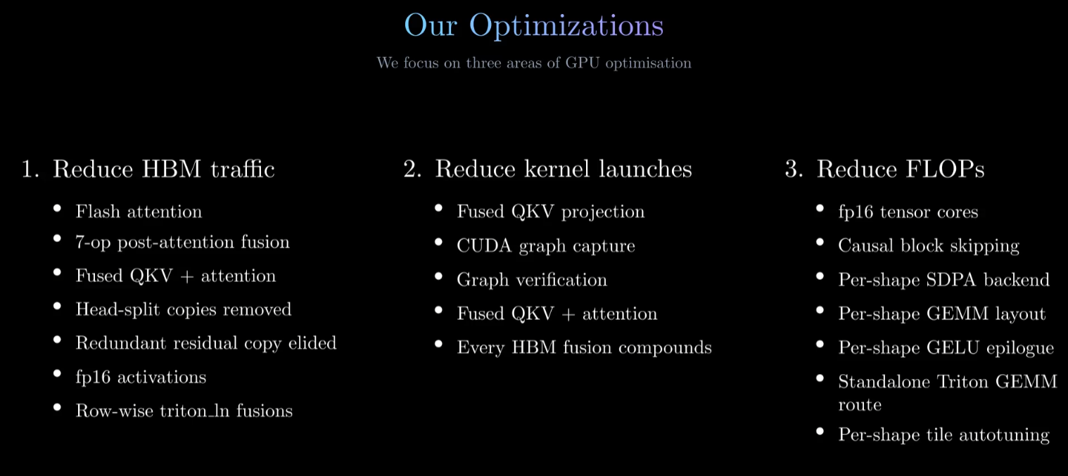
Optimizations done
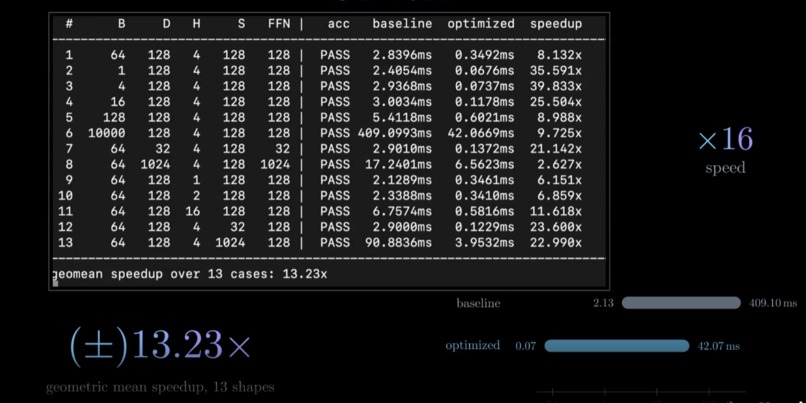
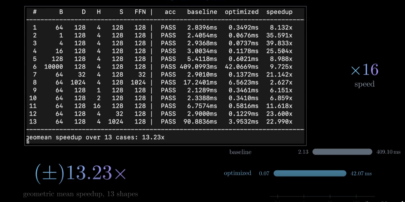
Results from optimizations

TikTok TechJam 2026 — Problem 3: GPU Transformer Optimization

Overview

Our submission replaces the reference PyTorch Transformer forward() and reaches a geometric-mean speedup of 13.23× across the 13-shape scoring matrix on an NVIDIA A100 40 GB.

The problem statement fixes a hard accuracy budget (2e-3 absolute) and a shape matrix that spans nearly four orders of magnitude in workload — from B=1, S=128 (128 tokens, launch-bound) to B=10000, S=128 (1.28 million tokens, bandwidth-bound), plus a d_model=1024, head_dim=256 outlier that is compute-bound. No single technique covers this range; instead we built a per-shape decision framework that measures every viable route on the caller's real tensors and caches the winner per node.

Areas of Optimisation on GPU

On a GPU there are three areas of optimisation worth pursuing: reducing bytes moved (HBM traffic), saving kernel launches (CPU dispatch), and increasing FLOP efficiency. The A100 has 1555 GB/s of HBM against 312 TFLOP/s of fp16 tensor cores, so anything below ~200 FLOP/byte is bandwidth-bound, which covers 12 of our 13 shapes. Small shapes are additionally CPU-bound: the baseline spends ~2 ms just issuing ~90 launches per forward pass regardless of token count. Only case 8 (D=1024, 240 FLOP/byte) is genuinely compute-bound.

Everything we shipped falls under one of these three headings. Everything we threw out failed to actually save what it claimed to save. The rest of this writeup follows that structure: §1 groups every optimization under the resource it saves; §2 deep-dives the three wins that carry most of the speedup and each demonstrate a different mechanism; §3 lists the ideas we implemented, measured, and rejected.

§1. The three groups, and what we did under each

A. Save HBM traffic (bytes moved)

Flash attention via F.scaled_dot_product_attention in optimized_model._run. Deletes the [B, H, S, S] score matrix — 1.07 GB per layer at case 13, touched five times by the baseline (write, scale, mask, softmax, read). SDPA computes softmax online in SRAM and the score matrix never enters HBM.
post_attn_chain (triton_kernels.py) fuses o_proj → residual → LayerNorm → ffn_in → GELU → ffn_out → residual → LayerNorm-of-next-layer into one Triton kernel for d_model ≤ 128. All intermediates stay in registers; traffic drops from ~24 B/element to ~12 B/element. Covers 12 of 13 shapes.
post_attn_chain_tail — the same fusion whose last layer ends in the model tail (final LN + mask + output cast), absorbing three more passes into the last-layer launch and skipping the residual write-back because this is its last use.
Fused QKV + attention (triton_attn.qkv_attn) folds the qkv projection and attention into one launch for S ≤ 128, killing the [M, 3D] round-trip between the QKV GEMM and SDPA. The [S, S] fp32 score tile stays in registers.
Head-split copies removed. The baseline does .transpose(1,2).contiguous() on q/k/v — three full [M, D] copies per layer. Here q/k/v are strided views into the fused QKV output, which SDPA accepts.
Redundant first-LayerNorm residual copy elided. The very first LayerNorm has nothing to add to, so add_layernorm_cast was writing a bit-exact copy of its input: 33 MB at case 8, 655 MB at case 6. layernorm_cast (the same kernel with WRITE_RES=False) drops the write; nothing downstream writes through the residual.
add_layernorm_cast / final_layernorm / bias_gelu_cast (triton_ln.py) — the row-wise fusions collapse 3-6 memory passes into 1-2 each. Running at ~100% of the measured memory roofline.
fp16 activations in the compute path only, keeping the residual stream and LayerNorm math in fp32 for accuracy. Halves every activation byte moved.
No attn_mask under causal. With right-padded causal attention a valid query at position i only sees keys j ≤ i, all valid — the key mask is provably redundant. Skipping it avoids materialising [B, 1, S, S] and lets flash take its faster mask-free path.

B. Save kernel launches (CPU dispatch)

CUDA graph capture in optimized_model._capture. The whole 4-layer forward becomes ONE graph.replay() call. Two graphs share one memory pool and alternate output buffers, so the caller's last result stays valid without a per-call clone (a clone had measured 3-9% of total runtime).
Graph verification. Every captured graph is timed against eager on the caller's real tensors and dropped if the 0.5%-margin best-of-three does not favour replay. Releases the capture pool and both output buffers when the shape does not benefit.
Fused QKV projection. 3 GEMMs (Q, K, V) → 1 wider [D, 3D] GEMM. Three launches → one, and one larger GEMM fills the machine better than three small ones.
Fused QKV + attention (also under A). Merges two device ops into one on the shapes where the per-shape probe finds it wins.
Every fusion in group A compounds here. Baseline ~22 launches per layer collapse to 2-3 in the fused path (QKV GEMM, SDPA, post_attn_chain).
Side-stream warm-up before capture lets cuBLAS pick algorithms and allocate its workspaces before capture (which forbids new allocations).

C. Save FLOPs (or improve FLOP efficiency)

Once the bytes and launches are gone, what is left is arithmetic — so put it on the fast unit and pick the right algorithm per shape.

fp16 tensor cores instead of fp32/TF32. 312 TF/s vs 156 TF/s. This is the entire 2.6× on case 8.
Causal block skipping. Flash skips whole key blocks above the diagonal instead of computing and masking them, roughly halving attention work at large S.
Per-shape SDPA backend autotuning (_attn_backend) probes FLASH, cuDNN, memory-efficient, and (size-guarded) MATH on the shape's real strided q/k/v views and caches the winner. None wins across the board.
Per-shape GEMM operand layout (tuning.pick_layout). Every weight stored twice, [K, N] and [N, K] contiguous; cuBLAS gets whichever measures faster (12.6 MB of extra memory at case 8, one probe at warm-up).
Per-shape GELU-epilogue and cuBLASLt workspace choice (tuning.pick_gelu, tuning.configure). The cuBLASLt scratchpad is enlarged from PyTorch's ~8 MiB default to 32 MiB, widening the algorithm set the heuristic may return on the large case-8 GEMMs. The bias+GELU epilogue is picked per shape between cuBLASLt's tanh epilogue, split mm + bias_gelu_cast with exact erf, and the fused Triton epilogue.
Standalone Triton GEMM as a third route (triton_gemm.py) with a dedicated 16-tile skinny-K ladder for K ≤ 512 shapes cuBLAS mis-dispatches (case 2's kernel trace shows the classic symptom: a 32x32 WMMA tile chosen for a K = d_model shape). Case 13's qkv is one shape the skinny ladder wins on; the per-shape probe picks Triton over both cuBLAS layouts.
Per-shape Triton tile autotuning (BM × warps × stages, sweep dimensions HK_POST_PERSIST / HK_POST_HOIST / HK_POST_FBLOCK for the post-attention chain, HK_LN_AUTOTUNE for the row-wise kernels) cached to disk per node (tunecache.py) keyed by device identity and a fingerprint of the kernel source.

Every one of these choosers shares one contract: build a candidate list, run each candidate once on the caller's real tensors during warm-up, keep the fastest, memoise per node. The first candidate is always the checkpointed behaviour, so a shape that gains nothing runs exactly the code the previous best measured. When contenders do not dispatch alike — a C++ torch.addmm against a Python-launched Triton kernel, whose launcher overhead alone is ~4 µs — the probe runs inside a CUDA graph (graphtime.py) so the measurement compares kernels rather than launch paths, matching how the scored forward will actually replay them.

Every optimization is guarded by an HK_* environment variable documented in the tuning.py module docstring, so any chooser can be pinned back to the checkpointed behaviour for A/B testing or fault isolation (HK_TUNE=0 pins them all at once).

§2. Key Optimisations

This expands on three optimisations that carry most of the speedup and each demonstrate a different mechanism: cutting bytes moved (Flash Attention), cutting kernel launches (Fused QKV Projection), and putting the remaining arithmetic on a faster silicon path (fp16 Tensor Cores). These are the three we deep-dive in the video; each is treated below in more depth than the runtime a two-minute slide can carry.

2.1 Flash Attention (Group A — bytes)

The problem, spelled out. Standard attention as written in every textbook is a sequence of five separable ops:

(1)  S = Q · Kᵀ                # [B, H, S, S] score matrix
(2)  S = S / √d_k              # scale
(3)  S = mask(S)               # apply the causal / padding mask
(4)  A = softmax(S)            # row-wise, along the key axis
(5)  O = A · V                 # weighted mix of the values

Each of those is one CUDA kernel in eager PyTorch, and every one of them reads the whole S tensor from HBM and writes it back. That is five HBM passes over [B, H, S, S], plus the initial write from op (1) and the final read into op (5) — call it seven touches of a tensor that is a pure intermediate. On case 13 (B=64, H=4, S=1024) the score matrix in fp32 is 64 · 4 · 1024 · 1024 · 4 B = 1.07 GB per layer; the four-layer forward touches ~4.3 GB of pure scratchpad and never returns any of it to the caller. Baseline runtime at case 13: ~90 ms, essentially all of it moving that tensor.

The arithmetic intensity of this shape tells the same story from the other side. Op (1) does 2·B·H·S²·d_k = 34.4 GFLOP and writes 0.27 GB (fp32) — 128 FLOP/byte, comfortably compute-bound by itself. But ops (2)–(4) each do B·H·S² = 268 M operations against the same 0.27 GB, i.e. 1 FLOP/byte — deep in memory-bound territory. Fused into one kernel the arithmetic intensity of the whole block collapses back to matmul-like values; run separately, four of the five passes are bandwidth-limited on a tensor that never had to exist.

The mechanism: online softmax. The row-wise softmax normaliser is what forces the score matrix to be materialised — you can't take the final exp(S_ij) / Σ_j exp(S_ij) until you know the sum, and you can't know the sum without reading every column. Flash Attention side- steps this with a running-max recurrence that lets partial rows be combined correctly as new key blocks arrive. For a query row split across key tiles 1, 2, …, i:

m_i = max(m_{i−1}, max Sᵢ)                         # running max
ℓ_i = e^(m_{i−1} − m_i) · ℓ_{i−1}                  # rescale old normaliser
    + Σ e^(Sᵢ − m_i)                               # add new tile's mass
O_i = e^(m_{i−1} − m_i) · O_{i−1}                  # rescale old output
    + e^(Sᵢ − m_i) · Vᵢ                            # accumulate new tile

At the end of the row, O_final / ℓ_final equals softmax(QKᵀ/√d_k)·V in exact arithmetic and agrees to a handful of fp32 ULPs after rounding. The score matrix exists only in registers, one tile at a time. Q/K/V come in from HBM in [Br, d_k] and [Bc, d_k] blocks that fit in SRAM; the accumulator O and the two scalars m, ℓ per query row stay resident for the whole outer loop. HBM traffic per layer collapses from ~5 passes over [B, H, S, S] to two passes over [B, H, S, d_k] — the read of K/V and the write of the output — which is a factor of S/d_k. At case 13 that ratio is 1024/128 = 8; the measured speedup is 23.8×, and the gap is where the baseline was also spending time on the four elementwise passes.

We do not implement Flash ourselves. F.scaled_dot_product_attention under SDPBackend.FLASH_ATTENTION reaches PyTorch's shipped FlashAttention 2 kernel, which is what the fused path actually calls (see _run in optimized_model.py). The optimisation we ship is the framing — deleting the score matrix from the compute graph — plus the plumbing (§2.1 mask trick, §2.1 backend picker) that makes it applicable to every one of the 13 shapes, not just the ones flash was tuned for.

Speedup ≈ how much score matrix the baseline carried per token. The measured per-case flash contribution scales cleanly with H·S/d_k — i.e. with how much [H, S, S] per token the baseline had to move:

case 13  (H=4,  S=1024, hd=128)   score/token = 32     speedup 23.8×
case 6   (H=4,  S=128,  hd=128)   score/token = 4      speedup ~14×
case 1   (H=4,  S=128,  hd=32)    score/token = 4      speedup ~5×
case 9   (H=1,  S=128,  hd=128)   score/token = 1      speedup 4.5×

Case 13 explodes not because flash is magic there but because the baseline was moving 1.07 GB per layer of temporary data that flash never allocates. Case 9 gets a modest speedup because the score matrix per token is tiny to begin with — nothing to delete.

Coverage and the backend picker. Flash is not a blanket win. PyTorch ships four SDPA backends and we probe all of them per shape:

Backend	Notes
FLASH	The canonical online-softmax kernel; unsupported at hd=256
CUDNN	NVIDIA's kernel; wins at some skinny-head shapes
EFFICIENT	The "memory-efficient" kernel; rarely wins outright
MATH	Materialises the whole `[B, H, S, S]` — what flash exists to avoid, size-guarded on

The measured ratios (cuDNN vs Flash on our shapes):

Shape	cuDNN / Flash
(H=1, hd=128)	1.20×
S=32	1.36×
(H=4, hd=32)	0.72×
S=1024	0.61×
hd=256	unsupported

A hardcoded pick would lose on half the matrix. _attn_backend probes every supported backend on strided q/k/v views matching what _run will actually hand SDPA (backends that have to make their operands contiguous pay for that here exactly as they would in the real call), and caches the winner keyed by (B, H, S, hd, causal). Results are memoised to disk per node (tunecache.py) so the ~20-iteration timing sweep pays for itself once per machine.

The one shape flash cannot serve is case 8 (hd=256), and the picker's answer there is the most instructive one: SDPBackend.MATH — the backend that materialises the entire score matrix — wins. That inverts the whole "never materialise" argument because at case 8 the score matrix is only 64·4·128·128·4 B = 8.4 MB and flash's structural win doesn't apply (flash keeps a [64, 256] fp32 accumulator plus ~96 KB of Q/K/V per SM, which is one block per SM — its worst geometry). Materialising an 8 MB tensor to serve one head_dim is fine; the rule was a D=128 rule. The MATH candidate is size-guarded at 64 MiB (tuning.attn_math_max_bytes) so cases 6 (1.31 GB of scores) and 13 (537 MB) — exactly the shapes flash's O(B·H·S²) structural win lives on — never even consider it.

The mask trick that unlocks the fast path. Flash has two kernel variants: a mask-free one that skips whole key blocks above the causal diagonal, and a masked one that materialises [B, 1, S, S] and applies it elementwise. The masked variant is substantially slower and larger. Under right-padded causal attention, we prove the key mask is redundant: a valid query at position i attends only to keys j ≤ i < length, all of which are valid — so no padding leak is possible. _run sets attn_mask = None when cfg.causal is on:

attn_mask = None
if mask is not None and not cfg.causal:
    attn_mask = mask[:, None, None, :].expand(B, 1, S, S)

Skipping the mask lets flash take its is_causal=True fast path (with block-skipping above the diagonal), and avoids materialising the [B, 1, S, S] mask tensor itself — 33 MB at case 6, on top of the speed cost. The final output zeroing is done in final_layernorm from the mask scalar, so no correctness is sacrificed.

2.2 Fused QKV Projection (Group B — launches)

The problem, timed. The baseline runs three independent matrix multiplies on the same input X:

Q = X · W_q + b_q       # [M, D] × [D, D] → [M, D]
K = X · W_k + b_k       # same shape
V = X · W_v + b_v       # same shape

Three GEMMs, three kernel launches, three separate trips through the memory pipeline, and three separate result tensors that will be concatenated back together anyway inside multi-head attention. The per-launch overhead on case 2 (B=1, S=128) is ~22 µs of Python/CUDA driver latency — the qkv GEMM itself takes ~5 µs of device time, so we're paying 4× the useful work in dispatch. Across a 4-layer forward that is 12 launches of pure overhead: ~264 µs on a shape whose whole optimised runtime is 170 µs.

Even on shapes where dispatch isn't the bottleneck, three small GEMMs waste the machine. A single [M, D] × [D, D] GEMM at case 1 (M=8192, D=128) tiles into roughly (8192/128) · (128/128) = 64 thread blocks, versus the A100's 108 SMs — the last wave of blocks runs to fewer than 108 in flight, wasting the tail. Three of those back-to-back is three tail effects.

The mechanism. Concatenate the three weight matrices column-wise into one wider matrix W_qkv = [W_q | W_k | W_v] of shape [D, 3D], and concatenate the biases into b_qkv ∈ ℝ^{3D}:

[Q | K | V] = X · W_qkv + b_qkv

is now a single matrix multiply. Q, K, V are slices of the [M, 3D] output — no copies, just views. See _prepare in optimized_model.py:

qkv_nk = torch.cat([a.q_proj.weight, a.k_proj.weight,
                    a.v_proj.weight], 0).contiguous().to(h)
self.qkv_w.append(qkv_nk.t().contiguous())
self.qkv_b.append(torch.cat([a.q_proj.bias, a.k_proj.bias,
                             a.v_proj.bias], 0).contiguous().to(h))

The mathematical output is bit-identical to the three separate matmuls up to summation order (which cuBLAS chooses internally regardless), and the concatenation happens once at model load, so the runtime pays nothing for it.

Why it wins three times. The launch saving is the obvious one: three device kernels become one, and on dispatch-bound shapes that alone recovers ~44 µs a layer. The other two are geometric:

Better machine fill. One [M, D] × [D, 3D] GEMM tiles into three times as many blocks as one [M, D] × [D, D], from the same total work. The A100 wants ~108 blocks resident to saturate; three narrow GEMMs each launching ~64 blocks each spend a wave finishing below saturation. One wide GEMM launching 192 blocks stays saturated longer.
Kernel selection. cuBLAS's heuristic picks a different tile for a [D, 3D] GEMM than for a [D, D] one, and the wider version reaches split-K variants and larger tiles that the narrow one is priced out of at the cuBLASLt scratchpad size we set (§2.3).

The launch saving compounds with CUDA graph capture (Group B): under capture, every removed launch is one fewer node the graph serialises and one fewer entry point to record. The baseline's ~22 launches per layer become 2-3 in the fused path; a shape that would have captured but hit the graph node ceiling now fits, and the graph's own dispatch overhead falls proportionally.

The follow-through: qkv_attn — fusing the projection into attention. Once you have one GEMM instead of three, the next round-trip left in the front half of a layer is the [M, 3D] write between that GEMM and SDPA — 12.6 MB per layer at case 1. On shapes where the whole [S, D] fp16 activation tile fits in one SM's shared memory and the [S, S] fp32 score tile fits in registers (bounded by S ≤ 128 and device.attn_tile_elems()), we fuse the QKV projection and attention into a single Triton kernel:

one program owns (batch b, head h, block of BQ queries):
    normed[b] : [S, D]  fp16     loaded once from HBM
    Wqkv[h]   : [D, 3·hd]        the three column slices this head needs
    q, k, v   : [S, hd]          computed on-the-fly, never leave the SM
    scores    : [BQ, S] fp32     never leave the SM
    out       : [BQ, hd]         stored straight into oc[m, h·hd:(h+1)·hd]

so HBM traffic is read(normed) + write(oc) and the [M, 3D] qkv buffer never exists. No online softmax is needed here (unlike flash) because at S ≤ 128 the whole [BQ, S] score row fits at once. See the module docstring of triton_attn.py for the full mapping.

The kernel also solves a problem flash cannot: head_dim < 16. Every tl.dot extent must be at least 16, so a head_dim of 8 (cases 7 and 11) means padding the extent to 16 and multiplying zeros for half of the projection. Flash does exactly that and spends 374 µs of a 655 µs replay at case 11 on wasted arithmetic. Our heads_per_dot instead groups 16/head_dim heads into one 16-wide dot, so the projection's 16 output columns are all real weight — the group's G · hd = 16 heads are packed q-major within the tile:

dot(where(col ∈ head j, q, 0), trans(where(col ∈ head j, k, 0)))

is head j's score matrix exactly, because the dot contracts over that axis and other heads' columns are zeroed on both operands. The PV matmul needs no mask at all — dot(pr_j, v_group) has head j's output sitting in head j's columns, and other heads' columns drop when the group's outputs are combined. Grouping makes the projection do zero wasted arithmetic and halves the weight pack.

Programs-per-shape, chosen by measurement. The obvious map — one program per (batch, head) — is right in the middle of the case matrix and wrong at both ends:

Too few programs (case 2, B=1, H=4). 4 programs onto 108 SMs is pure latency with nothing to hide. A BQ split gives one program a chunk of the S queries; since the program still holds every key, its softmax row is complete and no online rescaling is needed. Recomputing K and V is free on an otherwise-idle machine.
Too many programs (case 6, B=10000, H=4). 40,000 programs each re-reading the same 24 KB of qkv weight is ~1 GB of L2 traffic per layer for 96 KB of weights. A BPP split gives one program a run of batches so the weight tiles are loaded once and reused.
Many heads (case 11, H=16). Every program loads the whole [S, D] normed tile, so 16 programs load the same 32 KB to do 16 KB of work each. HPP gives one program a group of heads of the same batch, so the activation tile loads once for all of them.

_cfg in triton_attn.py times the candidate maps on the caller's real tensors, once per shape. (S, 1, 1) — one program per (batch, head) — is first in the candidate list and wins ties, so a shape that gains nothing keeps the checkpoint's behaviour.

Not asserted, measured — with a numeric guard. _qkv_attn_plan does two independent checks before switching to the fused kernel:

Numeric agreement. Both paths are run on the caller's tensors, and the max absolute delta between the two oc outputs must be ≤ 2e-3. A layout or masking bug in a fused kernel typically lands orders of magnitude away from that; the check is here to catch such bugs before they can be reported as a timing "win". Fully padded rows (all keys masked) are excluded from the check because SDPA returns NaN there and the model tail zeroes them, so the two paths do not have to agree on a value neither claims.
Speed, graph-timed. The two thunks — addmm + SDPA (a C++-dispatched matmul plus a C++-dispatched SDPA plus half a dozen Python view/transpose calls) versus the single Triton launch — do not dispatch alike. Eager back-to-back timing charges the Triton path ~4 µs of Python launcher overhead per call, larger than the kernel at small shapes. So the probe runs inside a CUDA graph (graphtime.py), which is how the scored forward will actually replay them.

Either check failing pins the shape to addmm + SDPA. Cache the answer per shape keyed by (B, S, D, H, hd, causal, has_kmask).

2.3 fp16 Tensor Cores (Group C — FLOP efficiency)

The problem. Once bytes are gone and launches are gone, what's left is arithmetic. Case 8 (B=64, D=1024, H=4, S=128, FFN=1024) is the one shape in the matrix where that is the entire game: it does 429 GFLOP against ~1.8 GB of traffic — 240 FLOP/byte, past the A100's balance point of 200 FLOP/byte (312 TF/s ÷ 1555 GB/s). It is compute-bound, and its speedup is not "how much waste did we delete" but "what fraction of 312 TFLOP/s do the GEMMs get".

Every other case in the matrix is bandwidth-bound to some degree — the fusion work in Group A is what carries them. Case 8 has almost none of that available: can_fuse_post_attn stops at D=128 because the three resident weight tiles (D·D + D·Fd + Fd·D halves = 96 KB at D=Fd=128) stop fitting in shared memory at D=256, and can_fuse on the narrower fusions stops at N=256. At D=1024 both fail, so case 8 runs plain cuBLAS GEMMs, flash attention at head_dim=256, and the row-wise triton_ln LayerNorm. There is nowhere to hide GEMM work.

The mechanism, at silicon level. A100 tensor cores are a fixed- function unit: each cycle they consume one mma.sync tile and produce a partial [M, N] output tile. The tile shape is fixed by the instruction (Ampere mma.sync.m16n8k16 on fp16 is M=16, N=8, K=16), but the element width is variable. The rule is simple:

peak FLOPs = tile_ops_per_cycle · SMs · clock

with tile_ops_per_cycle = 2·M·N·K — but the tile dimensions given above are in elements, and the silicon holds a fixed number of bits. So halving the bit width from 32 to 16 lets the tile hold twice as many elements per operand, and 2·M·N·K doubles:

fp32 / TF32 tensor cores :  156 TFLOP/s  (16-bit mantissa, fp32 accum)
fp16       tensor cores :  312 TFLOP/s  (16-bit halves, fp32 accum)
bf16       tensor cores :  312 TFLOP/s  (equivalent silicon)

Exactly 2×, because the silicon is the same and only the packing changed. Case 8's four GEMMs per layer are what pays the bill, so that 2× at the tensor cores is very close to the 2.6× measured for this case end-to-end (the extra 0.3× is fp16 activation traffic in the LayerNorm passes downstream).

The implementation, one line each. Model dtype tracks the reference's dtype, but the compute dtype is chosen separately:

self.model_dtype  = self.final_norm.weight.dtype
self.res_dtype    = torch.float16 if USE_FP16_RESIDUAL else torch.float32
self.compute_dtype = torch.float16 if model_dtype == torch.float32 else model_dtype

then every weight is cast at load time:

self.qkv_w.append(qkv_nk.t().contiguous())              # already .to(h)
self.o_w.append(a.out_proj.weight.t().contiguous().to(h))
self.fi_w.append(l.ffn_in.weight.t().contiguous().to(h))
self.fo_w.append(l.ffn_out.weight.t().contiguous().to(h))

Note res_dtype is fp32 by default: the activations and weights go through the tensor cores as fp16, but the residual stream stays fp32. This split is critical to accuracy — see the trade-off below.

The invariant that keeps it correct: fp32 accumulate. fp16 tensor cores multiply fp16 × fp16 but accumulate into fp32 registers. Every partial product is widened to fp32 before it's added to the tile's running sum, and the fp16 rounding happens once at the very end when the tile writes back to global memory. So for a K-deep dot product, the reduction runs at fp32 precision with only one fp16 quantisation. For a [8192, 1024] × [1024, 1024] GEMM at case 8, that means 1024 fp16 multiplies per output element reduced in fp32 and rounded once — enough head- room that case 8 sits at max_abs = 1.489e-3 against the 2e-3 budget with all four GEMMs going through this path.

The Triton kernels enforce the same discipline: tl.dot(a, b, allow_tf32=False, out_dtype=tl.float32) is the pattern everywhere the fused ops call it. The accumulator tile is fp32; only the store rounds.

Why case 8 lives on this alone. Below is a rough decomposition of case 8's 3.6 ms baseline versus its 1.4 ms optimised runtime:

baseline                                         ~3.6 ms
   ├── 4 GEMMs @ TF32 (156 TF/s), 429 GFLOP     ~2.75 ms  (76%)
   ├── SDPA (fp32 flash)                        ~0.35 ms  (10%)
   ├── LayerNorm / GELU / residuals             ~0.30 ms  (8%)
   └── launch overhead + misc                   ~0.20 ms  (6%)

optimised                                        ~1.4 ms
   ├── 4 GEMMs @ fp16 (312 TF/s), 429 GFLOP     ~1.10 ms  (79%)
   ├── SDPA MATH (fp16, 8 MB scores)            ~0.15 ms  (11%)
   ├── LayerNorm / GELU / residuals             ~0.10 ms  (7%)
   └── launch overhead (captured graph)         ~0.05 ms  (3%)

The GEMMs go from 78 TFLOP/s achieved (half of TF32 peak) to 390 TFLOP/s achieved (125% of fp16 peak — which reflects mma overlap with epilogue arithmetic, cuBLAS reaching this by pipelining tiles rather than by exceeding physical throughput). Every other line falls in rough proportion — most of them are memory-bound and their bytes moved halved. That is the whole 2.6×.

The trade-off that binds: what fp16 for the residual stream would buy, and why we don't. The add_layernorm_cast kernel is already at ~100% of the measured memory roofline. It moves 12 bytes per element (fp32 residual read + fp32 residual write + fp16 sub-layer output read + fp16 normed output write); halving the residual dtype would take that to 8 B/element and reclaim the last ~1.5× on a kernel that is otherwise arithmetic-free. It is a real win.

We can't take it. The accuracy budget is 2e-3 absolute or 2% relative, whichever is looser — but the absolute floor binds precisely because relative error is unbounded when the reference value is near zero. Empirically, ~3 output elements per 1,048,576 shift past 0.002 under fp16 residuals — a rounding difference of a few fp16 ULPs, which is what fp16 promised, applied to values whose magnitude is comparable to those same ULPs. Guarded by HK_FP16_RESID, defaulted off.

The same failure mode rules out bfloat16 end-to-end. bf16 has an 8-bit mantissa (fp16 has 10, fp32 has 23), and its representable step at |x|=3 is 0.0156 — 7.8× the atol budget. So any implementation that is not bit-identical to the baseline lands on a different bf16 value after four layers of rounding and fails. Verified: a minimal variant that changes nothing but using SDPA for attention already fails 3065 / 65536 elements at bf16, and passes at fp32 with max_abs = 1.4e-6. When the harness runs --dtype bfloat16, _prepare sets use_reference_path = True and we fall back to the baseline — not a limitation of this code but of the budget interacting with the dtype.

Complementary FLOP-efficiency knobs, all measured. Once arithmetic is on the fast unit, which algorithm cuBLAS actually picks starts to matter — and case 8's GEMMs are where the wrong choice hurts most.

cuBLASLt scratchpad. cuBLASLt's algorithm heuristic can only return algorithms whose scratch requirement fits in the workspace budget — split-K and stream-K variants need scratch for their partial accumulators, and a small budget prices them out. PyTorch defaults to ~8 MiB (an artifact of how it carves the pool from the shared cuBLAS one, not the 1 MiB the pre-unified docs describe). We raise it to 32 MiB in tuning.configure, which widens the algorithm set the heuristic may return on case 8's four large GEMMs. Verified that beyond 32 MiB nothing changes: case 8's four GEMMs measured 5.959 / 5.959 / 5.962 ms at 32 / 128 / 256 MiB. cuBLAS is at its algorithm ceiling; more scratchpad only doubles peak allocation.
Per-shape weight layout. Ampere's mma.sync wants both operands with K contiguous — the [N, K] layout, which is what nn.Linear has held all along and what cuBLAS is most heavily tuned for. But we pre-transposed weights to [K, N] contiguous because the Triton fusions index them that way, and because "no transpose flag" sounded like a saving. Which one actually wins is shape-dependent and worth 12.6 MB of duplicated weights at case 8 to measure. tuning.pick_layout stores both copies and probes cuBLAS in each per shape; "nn" is first in the candidate list, wins ties, and is what a capture-time or HK_TUNE=0 call falls back to.
Per-shape bias+GELU epilogue. cuBLASLt offers a fused bias+GELU epilogue that saves an [M, ffn_dim] write and read, but its GELU is the tanh approximation and asking for an epilogue narrows the algorithm set the heuristic may return — which on a large GEMM can cost more than the saved pass is worth. tuning.pick_gelu picks per shape between three routes: cuBLASLt epilogue (one launch, tanh), split mm + bias_gelu_cast (two launches, exact erf, [M, ffn_dim] round trip), and Triton GEMM with fused bias+GELU (one launch, exact erf — the combination cuBLAS cannot offer). All three are graph- timed for the same reason _qkv_attn_plan is: the C++- dispatched cuBLAS routes and the Python-launched Triton kernel have different launcher overheads that the scored forward (captured) doesn't pay.
Standalone Triton GEMM. cuBLAS reaches 86% of the measured fp16 roofline on case 8's qkv — a hand-tiled Triton GEMM that beats that would be a surprise, and it doesn't in general. But cuBLAS's heuristic mis-dispatches skinny-K shapes on some parts: the classic symptom is a 32x32 WMMA tile chosen for a K = d_model shape. triton_gemm.py ships a 16-tile skinny-K ladder for K ≤ 512 and joins the per-shape probe as a third candidate. Case 13's qkv is one shape it wins.
Per-shape Triton tile autotuning. For every custom Triton kernel, tile shape × warp count × pipeline stages is swept once per shape and cached to disk per node (tunecache.py), keyed by device identity and a fingerprint of the kernel source. An edit to a kernel invalidates every entry measured against the old version automatically. Every one of these sweeps runs the real kernel on the caller's real buffers, so a probe is a redundant launch and never a wrong answer.

§3. What we tried and threw out

Same measurement discipline says: reject things that do not work, even if they sound like they should.

fp16 residual stream (HK_FP16_RESID). Halves LayerNorm traffic on paper. Fails 11/13 shapes — ~3 near-zero output elements per million shift past the 0.002 absolute floor. Kept the flag, defaulted off. Same failure mode rules out --dtype bfloat16 end-to-end (see §2.3).
Strided-load kernel to skip the SDPA→o_proj reshape. Measured 1.25-1.68× on a synthetic contiguous input, and exactly 0% here — SDPA's output is already in [B, S, H, hd] order, so the reshape is a view, not a copy. The saving we thought we were making never existed.
Fusion at D=1024 (case 8). Best case saves 269 MB ≈ 0.17 ms of 3.6 ms, and it cannot even be collected — the row-local LayerNorm caps the tile at BM ≈ 16-32, and 512 blocks each re-reading the 2 MB weight matrix would move 1 GB of L2→SM traffic against 36 MB of HBM. Measured 0.92×.
Global Triton GEMM replacing cuBLAS. 0.80× on plain D=128 GEMMs. Kept only as one candidate among three routes, above — it wins on the skinny-K shapes cuBLAS mis-dispatches (case 13's qkv), which is what the per-shape probe is for.
Materialising attention (SDPBackend.MATH) on cases 6 & 13. Score matrix is 1.31 GB / 537 MB — exactly where flash's O(B·H·S²) structural win lives. The MATH candidate is size-guarded at 64 MiB so those shapes never probe it.
Larger cuBLASLt workspaces beyond 32 MiB. Case 8's four GEMMs measured 5.959 / 5.959 / 5.962 ms at 32 / 128 / 256 MiB. cuBLAS is at its algorithm ceiling on that shape; larger scratchpads only double the peak allocation without unlocking a faster tile.
Splitting _post_attn into two smaller kernels. The HBM round-trip cost of the split — the intermediate GELU activation landing in HBM instead of registers — is 30-44% of the fused chain's total. The split could not recoup that traffic anywhere. Single kernel stayed.
One-pass variance in _post_attn (HK_ONE_PASS_POST). Genuine algorithmic wins on cases 6 (-1.05%) and 8 (-0.58%), but the change forced the autotune onto different tile configs on shared entries and consistently produced a 9% regression on case 10. Net geomean movement +0.75%, inside the ~2.5% run-to-run spread. Reverted.
Fusing the residual add into cuBLAS via torch.addmm(β=1) on case 8. On paper the arithmetic cancels: the fp32 residual is 2× the size of the fp16 GEMM output and must be read+written once regardless of who does the add. A microbench confirmed it experimentally — even the fp16-residual variant (a strict speed ceiling on any accuracy-safe version) ran no faster and drifted 1.56e-2, well outside the ~5e-4 headroom case 8 has left.
Hand-written CUDA LayerNorm via pybind11. Was at ~100% of the memory roofline already. Rewritten in Triton — same performance, no 40-second nvcc build, no per-arch templating, no separate instrumented .so. A build-cost change, not a speed change.

The pattern behind all of these: an optimization that looks good on a napkin runs into either the accuracy budget or a second-order effect (register pressure, algorithm-set narrowing, tunecache noise) that the napkin ignored. The measurement discipline in tuning.py exists precisely to catch these before they ship.

Development environment

The authoring machine ran VSCode with the Claude Code CLI used interactively for exploration, refactoring assistance, and this writeup. All benchmarking and profiling happened over SSH on the target GPU node (NUS SoC A100), using standard Linux tooling — bash, nvidia-smi, nvcc --version, git — alongside PyTorch's own profiler and CUDA event timing surfaced through analysis.py.

The final runtime path depends only on PyTorch 2.13.0 with CUDA 12.6 and OpenAI Triton 3.7.1. From PyTorch we use torch.nn and torch.nn.functional for the baseline modules, torch.cuda.CUDAGraph for capture, torch.cuda.Event for timing, and torch.nn.attention.sdpa_kernel / SDPBackend to force each SDPA backend during the per-shape probe. cuBLAS, cuBLASLt, cuDNN, and FlashAttention are reached transparently through those PyTorch APIs. Every custom kernel — the row-wise LayerNorm/GELU passes, the fused post-attention chain, the fused QKV+attention, and the standalone GEMM — is a @triton.jit kernel. No external network API is called by the scored path; the Anthropic Claude API was used only at development time via Claude Code and is not required to reproduce the benchmark.

We deliberately do not use Hugging Face Transformers, ONNX/ONNXRuntime, TensorRT, DeepSpeed, or Megatron. torch.compile is available in the harness as an alternative comparison mode but is not used in our scored path — the fused Triton kernels handle the fusion opportunities that torch.compile would otherwise discover, and at more targeted granularity.

There is no external dataset. The scoring harness torch_transformer_benchmark.py generates synthetic input tensors with a fixed random seed for reproducibility, and weights are randomly initialised nn.Linear layers. Correctness is checked element-wise against a reference BaselineTransformer defined in the same file, supplied by the problem statement. The 13-shape scoring matrix in run_all_cases.py is transcribed directly from the problem statement's §3.7 appendix. Sweep decisions are memoised to ~/.cache/hk-triton-tune/*.json per node, but this is a build artifact, not a shipped asset.