Preparing Dicke states on Google's Willow chip

Abstract

Our create_dicke_state takes the day's calibration data for Google's 105-qubit Willow processor, chooses which qubits to use, and returns a circuit that prepares the requested Dicke state exactly in the absence of noise, using only the gates the challenge allows. Before writing a single circuit we worked out what the judges' score actually rewards. We then built a simulator that scores circuits the way the judges do, changed one thing at a time, and kept only what measured better. Over the 25 cases with N ≤ 10 the expected total score went from 82.8 to 102.0 (a perfect state would get 218.7). On the organizers' three test pairs our final circuits lead every alternative we compared in our simulator, and the depth-only bonus went from 23.8 to 44.47. All numbers are simulated; nothing here has run on hardware.

---

1. Problem Statement

Qubits. A classical register of N bits holds one of 2ᴺ strings. A register of N qubits holds one number, an amplitude, for every string at once (for us these are always real), and the squares of the amplitudes add up to 1. Measuring every qubit returns string b with probability (amplitude of b)². Measuring cannot reveal the sign of an amplitude, but signs still matter: they decide what the state does under later operations.

Dicke states. The Dicke state \(D^N_n\) is the equal superposition of every N-bit string with exactly n ones:

$$\lvert D^N_n \rangle = \frac{1}{\sqrt{K}} \sum_{\mathrm{wt}(b) = n} \lvert b \rangle, \qquad K = \binom{N}{n}$$

Picture N coins showing exactly n heads, in every possible arrangement at once, all with the same weight and the same sign. For example, D⁴₂ is the six strings 0011, 0101, 0110, 1001, 1010, 1100, each with amplitude +1/√6. The case n = 1 is called the W state. Below, D¹⁰₅ means N = 10 and n = 5, and k = min(n, N − n).

The chip. Willow's qubits sit on a square grid, and only neighbouring qubits can interact. Any single-qubit rotation is allowed. The only two-qubit gate is the CZ, which flips the sign of |11⟩ and leaves |00⟩, |01⟩ and |10⟩ alone. A CZ fails roughly ten times as often as a single-qubit gate, so a circuit's main cost is its CZ count. Its second cost is depth (the number of time steps), because qubits that sit idle also decay. Qubits and couplers vary a lot in quality, and some are unavailable on any given day.

The rules. With noise switched off, the circuit must produce the target state exactly, signs included. The only allowed gates are CZ on calibrated couplers, single-qubit PhasedXZ on calibrated qubits, and reset. There is no classical feedback. A circuit may have at most 1,750 moments and must build in under 60 s.

The noise. There are four sources:

• Gate errors: each gate occasionally applies a random wrong operation.
• Energy decay (T₁): a 1 relaxes to 0.
• Dephasing (T_φ): an idle qubit slowly loses track of its sign.
• Readout errors: a 1 is misread as 0 about twice as often as the reverse.

---

2. Scoring

Each (N, n) case is run for 10,000 shots measured directly (the Z basis) and 10,000 shots measured after rotating every qubit (the X basis). The case scores S = 1/(z + x), and the case scores are added up. The judged cases are not disclosed.

z asks whether the histogram is flat. Shots with the wrong number of ones are discarded, and f is the fraction that survives. The K valid counts c_b are then compared with an even split using Pearson's chi-squared statistic:

$$z = \frac{\chi^2}{K f}, \qquad \chi^2 = \sum_{\mathrm{wt}(b) = n} \frac{(c_b - F/K)^2}{F/K}, \qquad F = 10^4 f$$

x asks whether the signs are right. The Z basis can't see signs, but the X basis can. For each set of j qubits, take the product of their ±1 outcomes and average it over shots. Then average over all sets of that size. Flipping the bits of a j-subset keeps a string at weight n exactly when half of the subset was ones. So the ideal value is 0 for odd j, and for even j it is

$$C_j^\star = \binom{j}{j/2} \binom{N-j}{n-j/2} \Big/ \binom{N}{n}$$

x adds up the squared relative errors of these averages for j = 1, …, M, using the absolute error where the ideal value is 0. M is undisclosed; we always report M = N, the strictest choice. Noise shrinks the correlators toward 0, so x measures how much coherence survived. One convenient consequence: averaged over all j-subsets, a single shot's contribution depends only on how many ones it has (a Krawtchouk polynomial). That makes scoring thousands of simulated runs cheap.

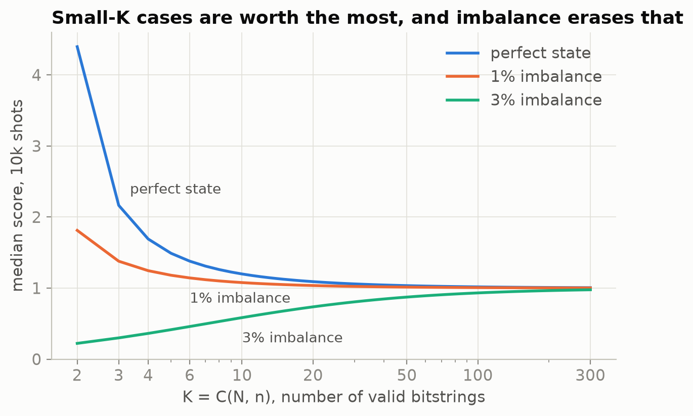
Finding 1: the score is heavy-tailed. For a perfect state, χ² follows a chi-squared distribution with K − 1 degrees of freedom. The score is the reciprocal of that random number, so it occasionally becomes huge. A short calculation gives \(\mathbb{E}[1/\chi^2_\nu] = 1/(\nu - 2)\) for ν > 2, and infinity for ν ≤ 2. For K ≤ 3 (W₂, W₃) only the small x term keeps the average finite. Expected score of a perfect state (f = 0.9, x = 0.001):

K	2	3	4	6	10	20
E[S]	51.4	8.15	3.34	1.79	1.28	1.06

A single K = 2 case is worth about fifty large ones.

Finding 2: imbalance erases that tail. Suppose valid string b appears with probability (1 + δ_b)/K instead of 1/K. Then χ² follows a noncentral chi-squared distribution, which can no longer land near 0. Its noncentrality is

$$\lambda = 10^4 f \cdot \overline{\delta^2}$$

A 1% rms imbalance cuts the K = 2 expected score from 51.4 to 33.3, and 3% cuts it to 1.3. Pre-tilting the amplitudes to cancel known biases is forbidden, because the noiseless state must be exact. Uniformity therefore has to come from the construction and from the choice of qubits.

Our priority order:

1. A valid circuit for every (N, n). Any valid circuit scores above 0, so we never refuse a case.
2. Uniformity and a low x floor on small-K cases.
3. A high kept fraction f. Leakage only costs linearly, through 1/f.
4. Coherence at large N.

The twist (Sun 04:01 ET). The organizers changed the preliminary ranking to 1/average(1/S) = 1/E[z + x], because the plain average blows up as noise vanishes, which is Finding 1. For large K,

$$\frac{1}{\mathbb{E}[z + x]} \approx \frac{1}{1/f + \lambda/(K f) + x}$$

Under this ranking total error (through f) and coherence (through x) decide, and imbalance enters only as λ/K. The notebook still describes final judging as one run per case on hardware, so we kept E[S] as our objective and report 1/E[z + x] alongside it.

---

3. Ideation

We set four ground rules on Saturday morning:

• Don't invent a new Dicke construction in 24 hours. We started from the literature: Bärtschi and Eidenbenz's deterministic recursion [1], with O(N) depth and O(nN) gates, and their later divide-and-conquer circuits [2]. The leverage is in engineering for this chip and this score.
• Build the measurement harness first, before any optimization.
• Get a baseline that is correct for every (N, n), before improving any one case.
• Change one thing at a time, and judge each change by the decomposed metrics, not the total alone.

Then we listed levers and tested each one:

Idea	Why it might help	What happened
Split the amplitude along a tree for W states	depth ~log N instead of N	Adopted. First sketched at 3 CZ per split; we showed 2 suffice and 1 is impossible
Numerically search for exact small circuits	routing B-E onto the grid wastes CZs on swaps	Adopted for N ≤ 8: D⁸₄ 162 → 27 CZ
Synthesize B-E's building blocks on a line of qubits	no routing at any N	Adopted as the general-N path
Calibration-aware placement	the best couplers are several times better than the median	Adopted
Dynamical decoupling (echo pulses on idle qubits)	protects idle qubits on hardware	Adopted, restricted to long idle windows
Among exact angle sets, pick the one least sensitive to over-rotation	systematic errors are missing from our noise model	Adopted
Schedule gates as late as possible (ALAP)	keeps qubits in the 0 state longer	Dropped: −1.4% to +0.1%
Mid-circuit measurement and feedforward (bonus)	divide and conquer	Dropped: the validator rejects classically controlled gates, and every scheme we costed was deeper at N ≤ 15
A GPU cluster	speed	Declined: the state vectors are tiny and the work is optimizer-bound

---

4. The evaluation harness

Every number in this writeup comes from a CSV this harness wrote (experiments/results/).

1. Calibrations. We use the challenge notebook's own random calibration generators with seeds 0–2. Anything we tuned was rechecked on held-out seeds 3–5.
2. Noise model (experiments/noise.py):
   • Depolarizing error after every CZ and every single-qubit gate, at its calibrated rate.
   • Idle decay with T₁ = 68 µs (Willow spec sheet) and T_φ = 100 µs (assumed), using 25 ns per single-qubit layer and 42 ns per CZ layer (assumed).
   • Asymmetric readout flips per qubit.
   • Two presets: gate (gate and readout errors only) and idle (gate and readout errors plus decay).
3. Simulation:
   • Exact density matrices up to N = 10.
   • Quantum trajectories (300 per case) for N = 11–15. We checked them against one exact D¹²₆ density matrix: median 0.255 from trajectories vs 0.260 exact.
4. Scoring:
   • The judges' overall_score, copied verbatim, plus a fast equivalent that agrees with it to 10⁻¹⁴ on identical shots.
   • 20,000 simulated 10,000-shot runs per case.
   • E[S], computed by integrating 1/(z + x) against the noncentral chi-squared density. It matches 10⁶-draw Monte Carlo. A plain average over resampled runs fails at K ≤ 3, where a few lucky draws dominate it.
5. What we report for every case:
   • E[S] (the objective)
   • median score
   • % of ceiling (relative to a perfect state)
   • f
   • χ²/(K − 1): equal to 1 when shot noise is the only effect, so anything above 1 is imbalance
   • x
   • 1/E[z + x]

Splitting the score this way tells us whether a loss is leakage (cut gates), imbalance (fix the construction or the qubits) or decoherence (cut depth).

1. Guardrails:
   • 419 tests:
     • an exact noiseless state;
     • a gate whitelist stricter than Willow105.validate_circuit;
     • the moment and build-time limits;
     • frozen "golden" circuits for N ≤ 8, so later changes can't silently alter them.
   • A hardening sweep of 969 builds, up to N = 105, with up to 15% of qubits dropped and with malformed calibration dictionaries.
   • The final notebook, scored with the notebook's own functions.

Not modeled: coherent (systematic) gate errors, which we study separately; ZZ crosstalk; leakage; per-qubit T₁ spread; and drift. Real hardware will score lower than everything reported here.

---

5. Architectures

Times are US Eastern, Oct 24–25. Totals are over the 25 cases with N ≤ 10, using the idle preset and 3 calibrations.

When (ET)	Change	Aimed at	Measured effect
Sat 12:45	v0 baseline: B-E routed onto the grid with cirq.RouteCQC; W states as a chain	valid everywhere	Σ E[S] 82.8, Σ median 22.2; D⁸₄ at 24% of ceiling
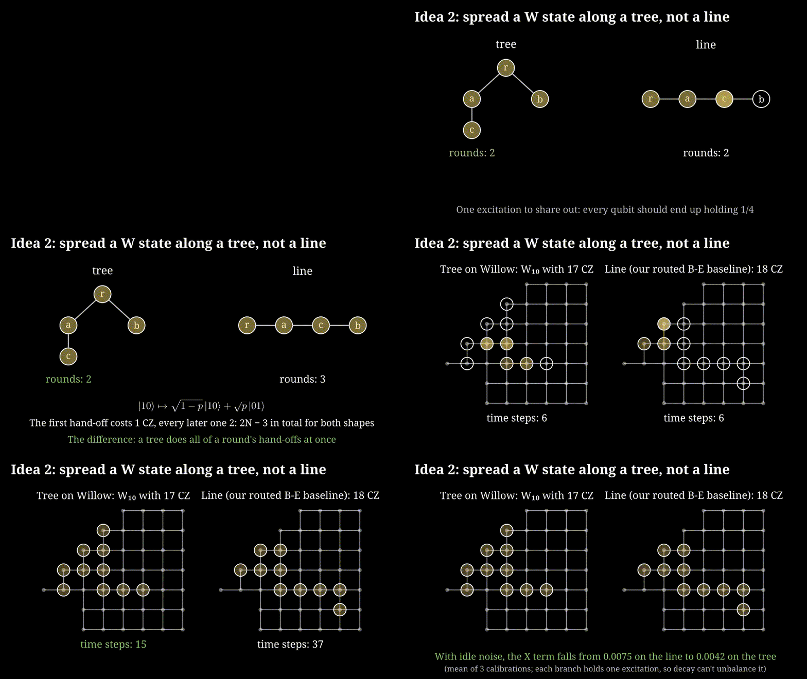
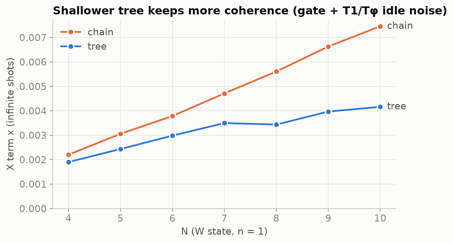
Sat 12:55	W states as a broadcast tree	depth → x	W₁₀ 37 → 15 moments, x 0.0075 → 0.0042
Sat 13:20–15:30	Exact whole-state synthesis, N ≤ 8	CZ count → f, x	D⁴₂ 21 → 5 CZ, D⁸₄ 162 → 27; D⁸₄ 24% → 77% of ceiling
Sat 14:00–16:30	B-E from synthesized line blocks, k ≤ 5	no routing	D¹⁰₅ 324 → 185 CZ
Sat 14:50	Dynamical decoupling only on idle windows of ≥ 4 slots	hardware dephasing	echoing every idle had cost up to 1 point of ceiling share in simulation
Sat 15:40	Robust angle picks	over-rotation imbalance λ	sensitivity 1.1–5.5× lower (D⁵₂: λ 50 → 9 at 1% over-rotation)
Sat 16:20	Objective switched to E[S]; W₂'s qubit pair chosen by predicted E[S]	heavy tail	W₂ +9% E[S] (−5% median, a deliberate trade)
Sat 16:50	Placement ranks every calibrated rate at value + 1σ	winner's curse	0 of 75 placements changed on the notebook's calibrations; a hedge for judging day
Sat 17:35	Portfolio with an independently developed "split B-E" solution, chosen per case by measurement	CZ count at k ≥ 2	Σ E[S] 101.0 → 102.0, Σ median 26.9 → 27.9; bonus 23.8 → 37.15
Sat 18:00–21:00	Big-N diagnosis; N = 9–10 synthesis on a 30-vCPU VM; trajectories to N = 15	large N	synthesis stops scaling (§8); D⁸₃ 43 → 31 CZ (+6.3% median, +6.7% on held-out seeds)
Sat ~22:10	Organizers' bonus feedback: 37.15 vs a leading 41.10	bonus depth	all 56 cases exact, so the gap was pure depth
Sun 00:30–04:00	Synthesized arm blocks; candidates ranked by depth	bonus depth	37.15 → 40.59 → 42.72 → 43.79
Sun 04:01	Organizers switch the preliminary ranking to 1/E[z + x]	—	we lead on D¹⁰₃, trail on D¹⁰₅ and D¹⁵₄
Sun 06:40–07:50	Exact single-qubit merge pass; three circuits from longer synthesis runs on PSC Bridges-2	single-qubit error budget	+1–11% (gate) / 0–21% (idle) at N ≥ 9; D⁷₃ 25 → 18 CZ; bonus 44.47
Sun 08:15	Final head-to-head against alternative combined notebooks; freeze	—	ours ahead on all six cases compared (D⁹₃–D¹⁰₅ by 2–10%, D¹⁵₄ by more); bonus 44.47 vs 44.27

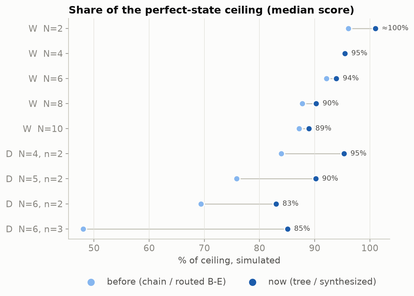
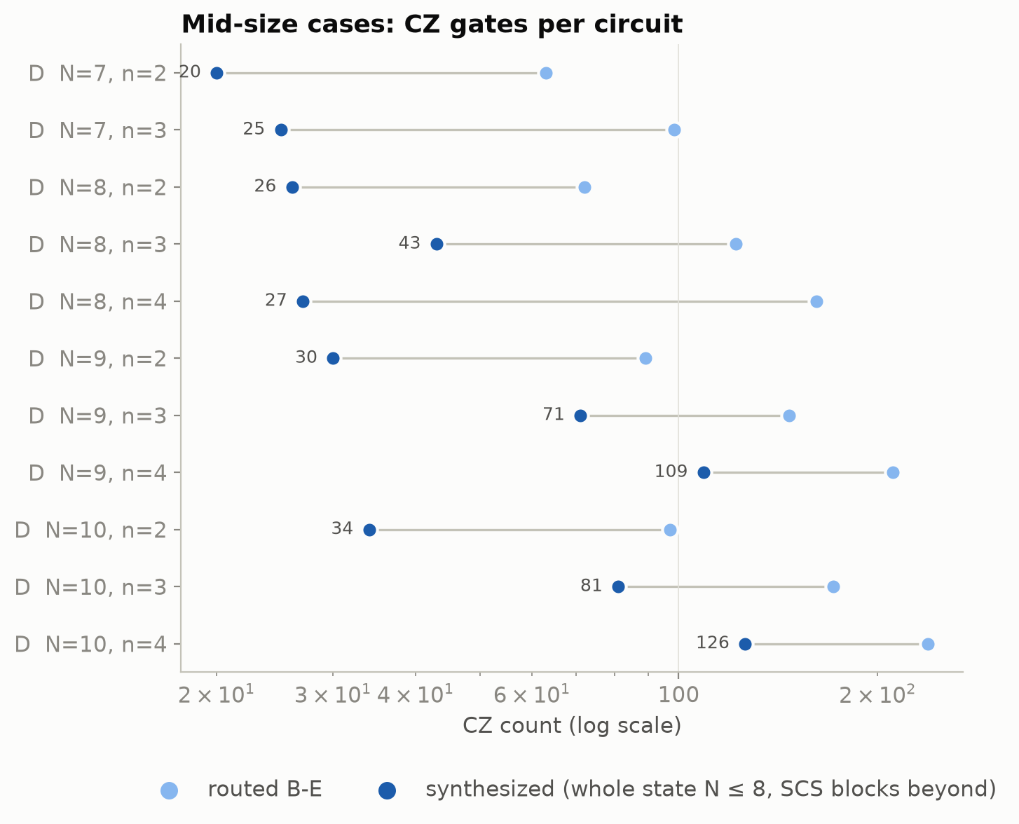
Both snapshots are from Saturday afternoon. Several of these cases improved further later (D⁸₃ 43 → 30 CZ, D⁷₃ 25 → 18).

Three turning points:

• The baseline diagnosis (Sat 12:45).
  • W states were already near their ceiling.
  • General n fell off quickly: D⁸₄ reached 24% of ceiling, and its x was as large as its z.
  • The loss was therefore gate count and coherence, not angles or symmetry. That made "fewer CZs" the first lever.
• Two solutions, one dispatcher (Sat 17:35).
  • Under the same harness, the split B-E (§6) won k = 2 at N ≥ 6 by 1–7% and k ≥ 3 at N ≥ 9 by 21–39% (D¹⁰₅: 85 vs 185 CZ).
  • Our constructions won the W states and the remaining small cases.
  • Rather than pick one, main.py sends each (N, n) to the measured winner.
• Answering the organizers (Sun).
  • Bonus feedback. All 56 of our cases were exact, so the gap was depth, and we profiled where it was (§6).
  • Revised ranking. It showed us trailing on D¹⁰₅ (0.358 vs 0.433) and D¹⁵₄ (0.398 vs 0.509). A per-gate error budget found that 60% of the single-qubit gates at N ≥ 9 were dense echo pulses. Under per-gate noise those pulses only add error: on D¹⁵₄ the single-qubit error budget matched the CZ budget (0.33 vs 0.27). An exact merge pass removed them.

---

6. Final architecture

create_dicke_state(N, n, calibration)
  k = min(n, N − n); if n > N/2, build D(N, N − n) and flip every qubit at the end
  ├─ k = 0                 → product state on the best-readout qubits
  ├─ k = 1                 → W broadcast tree (2N − 3 CZ)
  ├─ k = 2, N ≥ 6          → split B-E
  ├─ k ≥ 3, N ≥ 9          → split B-E
  ├─ N ≤ 8                 → exact synthesized circuit from a cached table, placed on the chip
  ├─ k ≤ 5                 → B-E from synthesized nearest-neighbour blocks on a path
  └─ otherwise             → B-E routed with cirq.RouteCQC on a low-error path
  then: exact single-qubit merge → XY4 echoes on long idle windows

Two free reductions.

• Complement. Flipping every bit maps weight-n strings to weight-(N − n) strings, so we only ever build k ≤ N/2.
• Placement and order. Swapping qubits leaves a Dicke state unchanged, and the answer is returned as a set of qubits. So a construction can go anywhere its shape fits, and routing never has to restore qubit order.

W tree (k = 1).

• Construction. One qubit starts in 1. In each round, every qubit that holds probability hands one neighbour exactly the share its subtree needs. Transfers run in parallel, so depth grows like log₂ N.
• Cost. The first transfer costs 1 CZ, and each later one is a 2-CZ rotation within the span of |01⟩ and |10⟩. One CZ cannot do a later transfer: it would have to leave |00⟩ unentangled but entangle |10⟩, and that is impossible. The total is 2N − 3 CZ, the same as a chain, but W₁₀ takes 15 moments instead of 37.
• Balance. Every branch carries one excitation throughout, so decay creates no imbalance.

Exact synthesis (N ≤ 8).

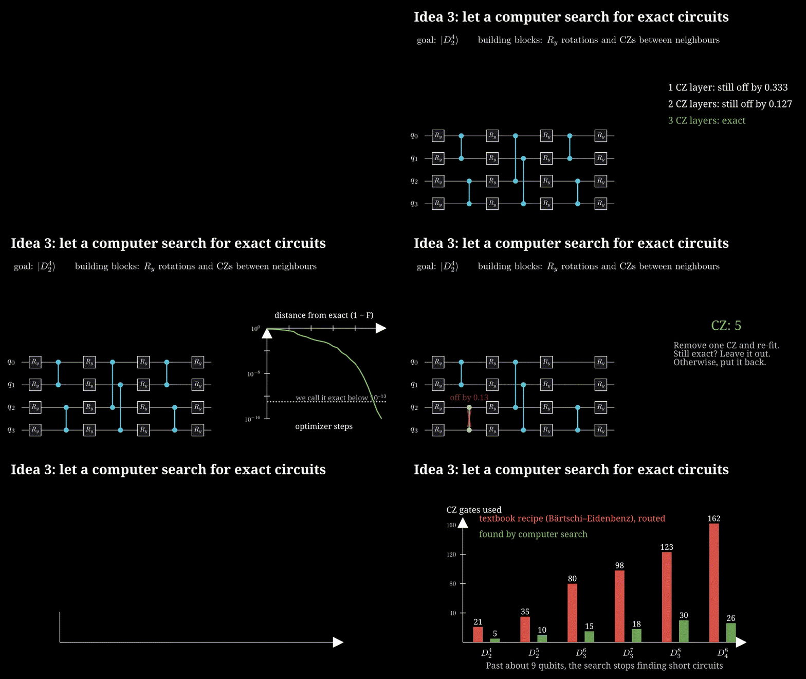
• Search space. Dicke amplitudes are real, so we search circuits of alternating R_y layers and brickwork CZs on a path or a 2×m patch. Given enough connectivity, this family reaches every real state [3].
• Search. L-BFGS with exact gradients drives the infidelity \(1 - \langle D^N_n \mid \psi(\theta) \rangle^2\) below 10⁻¹³. Greedy deletion then removes every CZ the circuit can do without while staying exact.
• Results. D⁴₂ 5 CZ, D⁵₂ 10, D⁶₃ 15, D⁷₃ 18, D⁸₃ 30, D⁸₄ 26, against 21–162 for routed B-E. The last three came from longer runs on PSC Bridges-2.
• Robust angles. One CZ pattern admits many exact angle sets. Over-rotation shifts probabilities at first order but a stray phase only at second order, so we deploy the set least sensitive to over-rotation (1.1–5.5× less).

Bärtschi–Eidenbenz (any N). B-E turns this identity into a sequence of "split and cyclic shift" blocks:

$$\lvert D^m_r \rangle = \sqrt{\tfrac{r}{m}} \lvert D_{r-1}^{m-1} \rangle \lvert 1 \rangle + \sqrt{\tfrac{m-r}{m}} \lvert D_{r}^{m-1} \rangle \lvert 0 \rangle$$

Each block only ever sees k + 1 sorted input strings, so it is a small isometry rather than a full unitary. We synthesize each block exactly on neighbouring qubits of a path, with every input mapped correctly with a common sign. The cost is 2, 4, 12, 17 and 29 CZ per block for k = 1–5, and no routing is needed.

Split B-E (k = 2 at N ≥ 6; k ≥ 3 at N ≥ 9). Split the qubits into arms of sizes a and b. The number of ones landing in the second arm is hypergeometric:

$$\lvert D^N_k \rangle = \sum_j \sqrt{P(j)} \lvert D^a_{k-j} \rangle \lvert D^b_j \rangle, \qquad P(j) = \binom{b}{j} \binom{a}{k-j} \Big/ \binom{N}{k}$$

The value j is written in unary, copied across, and both arms run nearest-neighbour B-E in parallel. A controlled rotation onto a qubit known to be 0 costs 1 CZ instead of 2, because R_y(θ/2) · Z · R_y(−θ/2) = R_y(θ) · Z and Z leaves 0 unchanged.

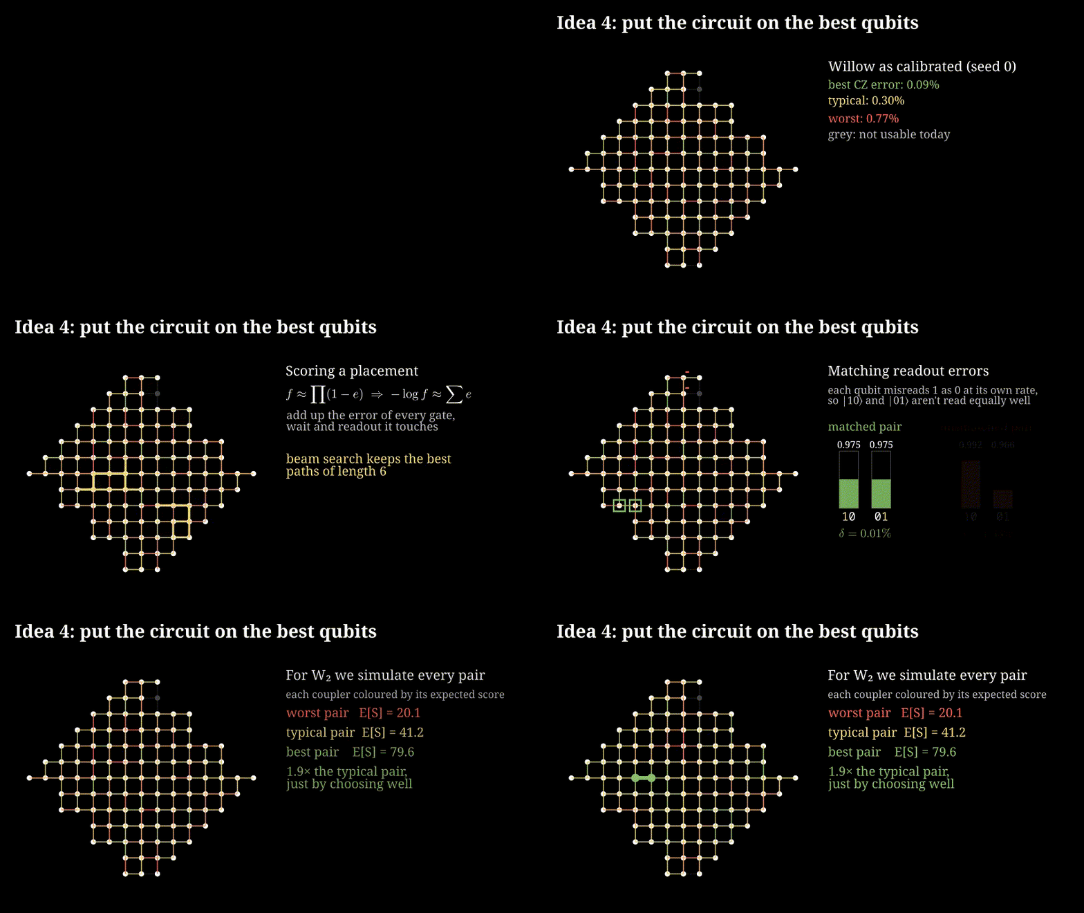
Placement. Every placement of a construction's shape on the calibrated grid is scored, and the lowest cost wins. The cost estimates log E[z]: since f ≈ Π(1 − e), −log f ≈ Σ e, so the cost is a sum over the circuit.

$$C = \sum_{\text{couplers}} u \cdot e_{\mathrm{CZ}} + \sum_{\text{qubits}} \left[ g \cdot e_{1q} + \left(1 - \tfrac{n}{N}\right) e_{0 \to 1} + \tfrac{n}{N} e_{1 \to 0} \right] + \tau \left( \tfrac{1}{T_1} + \tfrac{1}{T_\varphi} \right) + \log\left(1 + \tfrac{\lambda_{\mathrm{ro}}}{K - 1}\right)$$

• u and g count the gates on each coupler and qubit.
• Each qubit reads 1 with probability n/N, which weights its two readout error rates.
• τ is the total idle time.
• λ_ro is the imbalance caused by qubits that misread at different rates.
• Every rate enters as value + 1σ, so we don't favour qubits that only look good by chance.

Compilation.

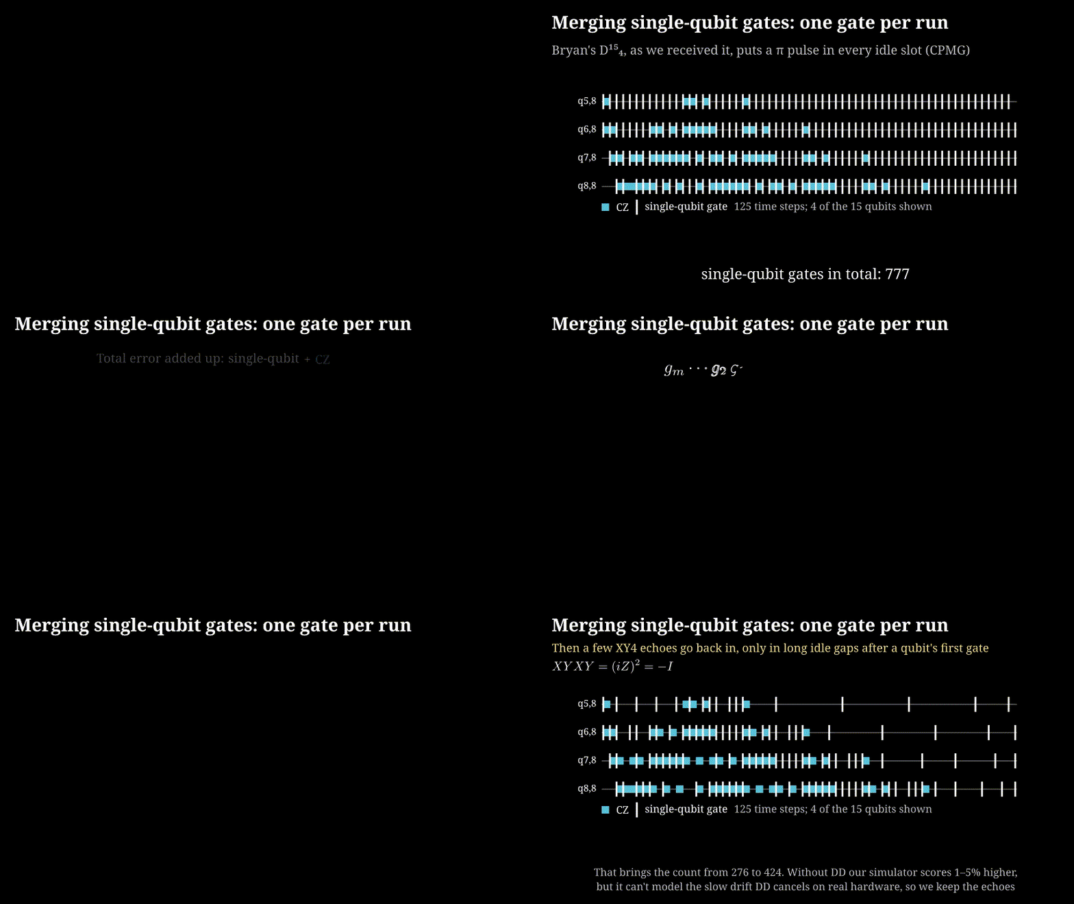
• Moments. Every moment is all-CZ or all-single-qubit.
• Merge pass. An exact pass folds each run of single-qubit gates into one PhasedXZ; D¹⁵₄ goes from 777 to 276 single-qubit gates.
• Echoes. We add XYXY echoes (product −I, so the noiseless state is unchanged) only in idle windows of 4 or more slots. Dropping them scores 1–5% better in simulation, but our memoryless dephasing model cannot show the slow drift they fix on hardware, so they stay.

Bonus entry (depth only). The bonus is scored by Σ N·n / moments over the 56 cases with 2 ≤ N ≤ 15 and 1 ≤ n ≤ ⌊N/2⌋.

• Unitary. Willow105.validate_circuit rejects classically controlled gates, so the entry uses none.
• Candidates. It builds every exact candidate and returns the shallowest.
• Where the depth was. In split circuits it sat in one arm's strictly serial tail: on D¹⁵₇, 147 of 160 moments.
• The fix. We replace that tail with one synthesized block \(U_{m_0} : \lvert 0^{m_0 - r} 1^r \rangle \mapsto \lvert D_r^{m_0} \rangle\). A 6-qubit arm with up to 4 ones drops from 97 moments to 43.
• Examples. D¹²₄ 88 → 51 moments, D⁹₃ 54 → 31, D¹⁵₇ 160 → 144.

---

7. Results

Final circuits (idle preset, 3 calibrations, M = N; arrows read "first baseline → final"):

case	K	construction	CZ	f	χ²/(K−1)	x	E[S]	% of ceiling
W₂	2	tree, best pair	2 → 1	0.990	1.041	0.0005	54.3 → 65.6	96 → 96
W₃	3	tree	4 → 3	0.977	1.026	0.0013	7.45 → 7.97	92 → 97
D⁴₂	6	synthesized	21 → 5	0.968	1.019	0.0058	1.55 → 1.85	84 → 95
D⁶₃	20	synthesized	80 → 15	0.923	1.014	0.0347	0.54 → 1.03	48 → 88
D⁸₃	56	synthesized	123 → 30	0.868	1.016	0.0958	0.39 → 0.83	38 → 79
D⁸₄	70	synthesized	162 → 26	0.880	1.019	0.1113	0.24 → 0.82	24 → 79
D¹⁰₂	45	split B-E	97 → 31	0.850	1.016	0.0438	0.38 → 0.86	36 → 81
D¹⁰₅	252	split B-E	324 → 85	0.692	1.046	0.8695	0.12 → 0.42	12 → 42

Totals. Over all 25 cases with N ≤ 10, the submitted notebook, scored with its own functions, gives:

• Σ E[S] = 102.0 and Σ median = 27.9.
• For comparison, a perfect state gives 218.7 and 33.1, and our first baseline gave 82.8 and 22.2.
• W₂ and W₃ alone hold about 73.5 of our expected total. That is why §2 drove the design.

The organizers' pairs under 1/E[z + x] (gate preset / idle preset, 3 calibrations; D¹⁵₄ from trajectories on one calibration):

case	K	before merge pass	final	our team's earlier preliminary entry
D¹⁰₃	120	0.765 / 0.639	0.776 / 0.639	0.722 / 0.582
D¹⁰₅	252	0.569 / 0.421	0.603 / 0.421	0.582 / 0.413
D¹⁵₄	1365	0.491 / 0.318	0.546 / 0.351	0.447 / 0.310

Our simulator does not reproduce the size of the gaps on the organizers' preliminary ranking, so read this table as a statement about our noise model.

Large N (trajectories, N = 11–15):

• W states stay at 82–89% of ceiling, but half filling falls to about 15%.
• Overall fidelity (~0.6–0.75) drives both terms, with z ≈ 1/f.
• Gates and idling matter about equally. D¹⁰₅ has a median of 0.53 with gate noise alone, 0.59 with decay alone, and 0.375 with both.

Bonus: score_solution = 44.47 over all 56 cases, each one exact, routed and whitelisted. The first-round feedback was 37.15, against a leading 41.10.

---

8. Unsuccessful attempts

• Whole-state synthesis at N = 9–10.
  • An overnight run with 24 workers found exact circuits with 33, 35, 98 and 136 CZ for D⁹₂, D¹⁰₂, D⁹₄ and D⁹₃. The deployed circuits use 27, 31, 63 and 50.
  • Random-start brickwork stops scaling around N ≈ 9.
• Compressing the split-B-E circuits. We re-parametrized them and deleted single CZs. Exactness came back 0 times in 8 (best residual 1.6 × 10⁻⁴).
• ALAP scheduling: −1.4% to +0.1%.
• Fewer CZs that measured worse.
  • A 14-CZ D⁶₃ lost to our 15-CZ one: its imbalance λ was 0.8–1.0 against 0.25.
  • At small K a lower λ is worth more than one CZ.
• Shallower bonus templates.
  • Excitation-preserving brickwork, 2D patches, and complex single-qubit layers all needed as many layers as R_y + CZ on a path, or more.
  • Splitting into more than two arms costs O(k) controlled rotations per thermometer bit. At N ≤ 15 that is about as much as it saves.

---

9. Lessons learned

• Analyze the metric before writing circuits. That analysis reordered our plan (small K first). It also predicted the instability that made the organizers change the aggregate.
• Decompose every score. f, χ²/(K − 1) and x each point to a different fix, and the total alone hides which one is needed.
• Fewer CZs is not automatically better, and neither is more echoing. Measure each change on the full score.
• Know where your simulator is blind. Ours misses coherent errors, crosstalk and drift. For those we hedged (robust angles, +1σ placement, sparse echoes) instead of tuning to the simulator.

What's next:

• Use hardware data on over-rotation and T₂* to settle the decoupling trade-off.
• Check whether mixed CZ + single-qubit moments behave as the model assumes.
• Find exact blocks for the k ≥ 5 bonus arms (12 cases, 8.0 points).
• Add per-qubit T₁ to placement.

---

10. Reproducibility

uv venv --python 3.12 .venv
uv pip install --python .venv/bin/python --prerelease=allow -r requirements.txt   # Willow105 needs the cirq 1.8 dev build
.venv/bin/python -m pytest tests/ -q                                              # exactness + rules, N <= 10, golden N <= 8
.venv/bin/python experiments/evaluate.py --out mine.csv --nmin 2 --nmax 8 --noise idle --repeats 20000
.venv/bin/python experiments/summarize.py mine.csv                                # f, chi2/(K-1), x, E\[S\], median, % of ceiling
.venv/bin/python experiments/bench_notebook.py --workers 28                       # submission.ipynb scored by its own functions

Links:

• Repository
• submission.ipynb, the entry
• ARCHITECTURE.md: every table, with its source CSV
• Website

References

[1] A. Bärtschi and S. Eidenbenz, "Deterministic Preparation of Dicke States," FCT 2019, arXiv:1904.07358.
[2] A. Bärtschi and S. Eidenbenz, "Short-Depth Circuits for Dicke State Preparation," IEEE QCE 2022, arXiv:2207.09998.
[3] M. Möttönen, J. J. Vartiainen, V. Bergholm, M. M. Salomaa, "Transformation of quantum states using uniformly controlled rotations," QIC 5 (2005), arXiv:quant-ph/0407010.
[4] Google Quantum AI, Willow processor spec sheet (2024).

Built With

• cursor
• google
• quantum