-
-
Company Logo
-
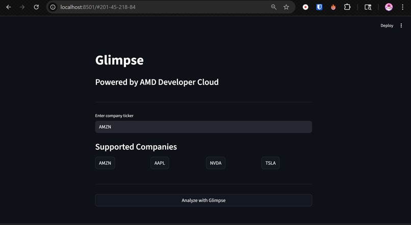
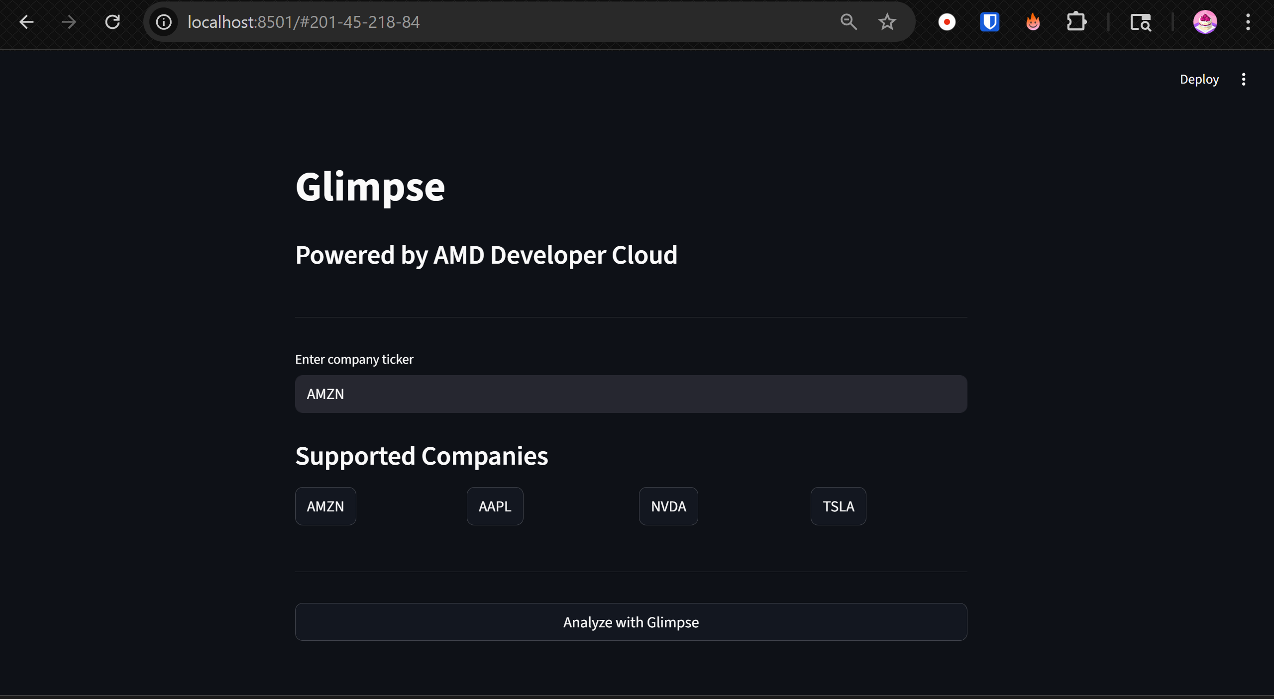
Home Page
-
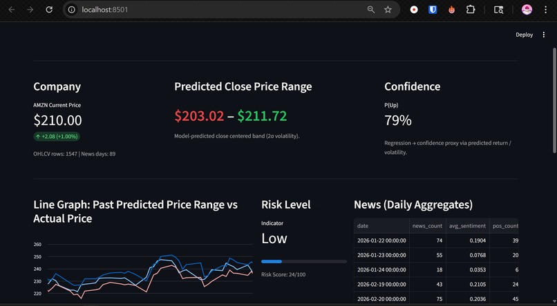
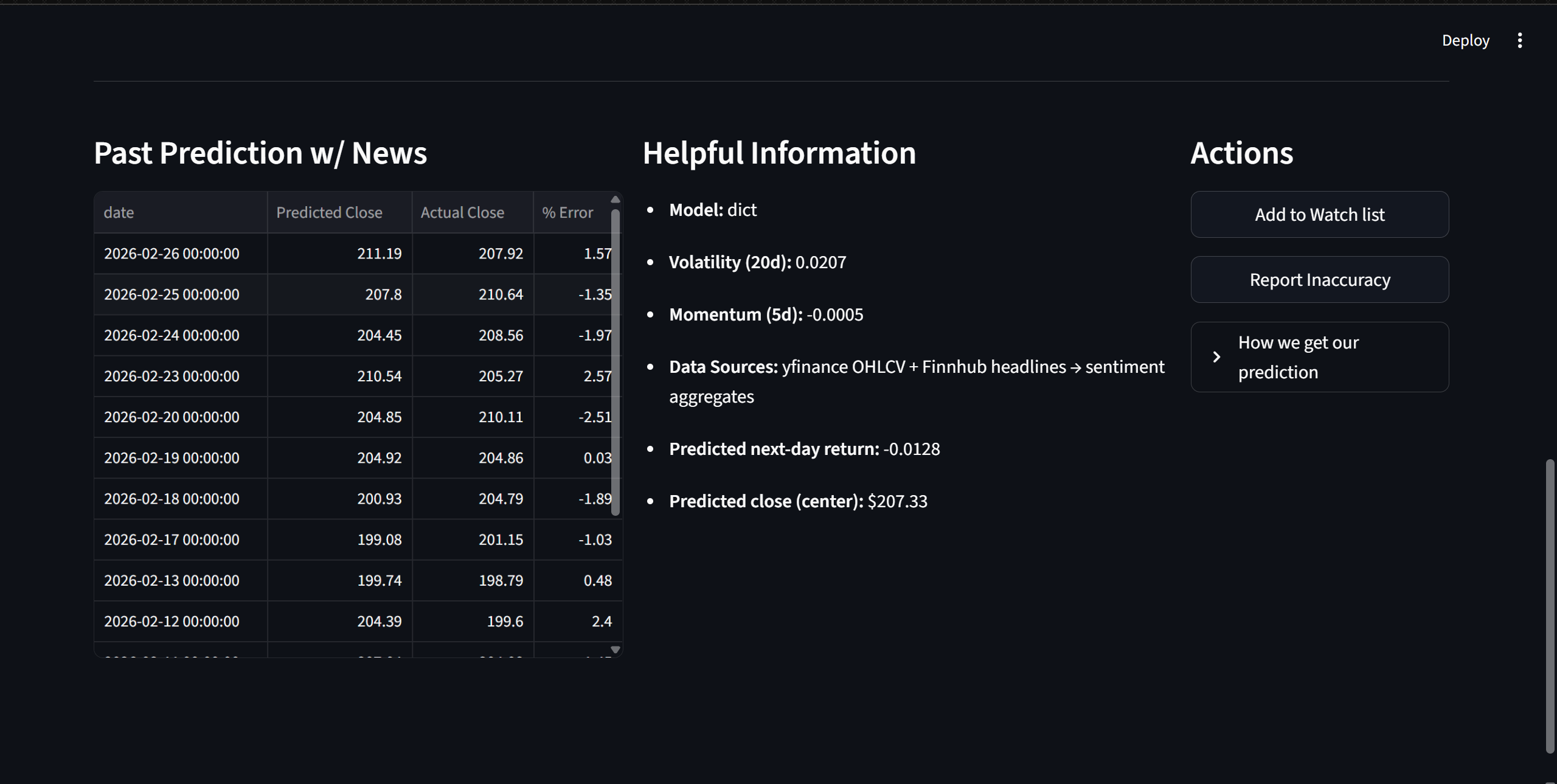
Dashboard
-
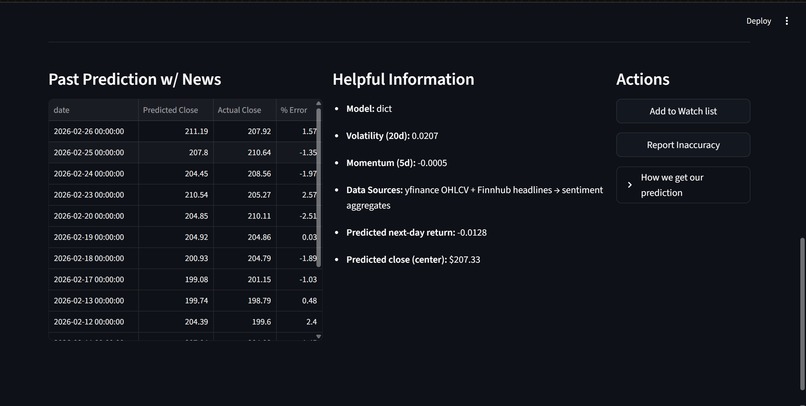
Dashboard
-
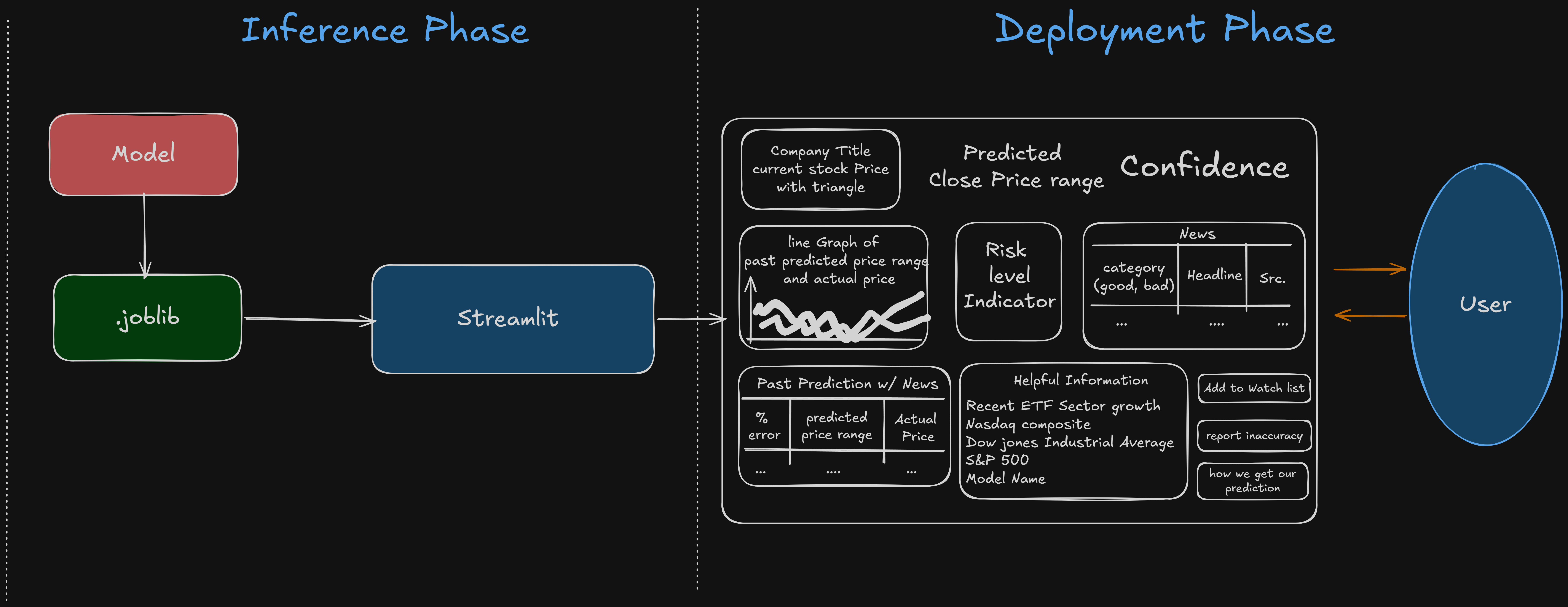
Architecture
-

Architecture
-

Page Layout
-
Page Layout
-
Intermediate Output


Glimpse: Probabilistic Next-Day Stock Price Range Forecasting
🚀 What Inspired Us
Financial markets are inherently uncertain. Most stock prediction tools output a single number — a point estimate of tomorrow’s price. But in reality, markets don’t move to a single deterministic value. They move within a range, influenced by volatility, sentiment, and macro events.
We were inspired by a simple question:
Instead of predicting one price, can we predict a probabilistic range for tomorrow’s close?
Rather than saying: [ \hat{P}_{t+1} = 208.34 ]
We wanted to say: [ P_{t+1} \in [203.02,\; 211.72] \quad \text{with approximately 80% confidence} ]
That shift — from point forecasting to uncertainty-aware forecasting — became the foundation of our project.
🧠 What We Built
We built Glimpse, a probabilistic next-day stock price range forecasting system.
Instead of predicting a single closing price, our system predicts:
[ Q_{0.10}(Y_{t+1} \mid X_t), \quad Q_{0.90}(Y_{t+1} \mid X_t) ]
Where:
- ( Y_{t+1} ) = next-day log return
- ( X_t ) = engineered features at time ( t )
- ( Q_{\alpha} ) = conditional quantile at level ( \alpha )
This gives us an 80% prediction interval:
[ \left[ \exp(Q_{0.10}) \cdot P_t,\; \exp(Q_{0.90}) \cdot P_t \right] ]
Where:
- ( P_t ) = today’s close price
- We model log-returns for stability and better tail behavior.
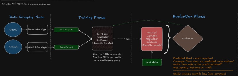
🔬 How We Built It
1️⃣ Data Pipeline
We combined two major data sources:
- OHLCV price data (via
yfinance) - News sentiment data (via Finnhub + VADER sentiment analysis)
We aggregated headlines daily and engineered features such as:
- Lagged returns
- Rolling volatility
- Moving averages
- Intraday spread
- Momentum
- News sentiment metrics
All news features were shifted by one day to avoid data leakage.
2️⃣ Feature Engineering
We constructed a feature matrix:
[ X_t = f(\text{price history}, \text{volatility}, \text{news sentiment}, \text{calendar}) ]
Our target variable:
[ Y_{t+1} = \log\left(\frac{P_{t+1}}{P_t}\right) ]
Using log returns instead of simple returns improves numerical stability and tail modeling.
3️⃣ Model Architecture
We trained two independent LightGBM quantile regression models:
- Model A: ( \alpha = 0.10 )
- Model B: ( \alpha = 0.90 )
Each model minimizes pinball loss:
[ L_\alpha(y, \hat{y}) = \begin{cases} \alpha (y - \hat{y}) & \text{if } y > \hat{y} \ (1 - \alpha)(\hat{y} - y) & \text{if } y \le \hat{y} \end{cases} ]
This allows us to directly estimate conditional quantiles instead of assuming normality.
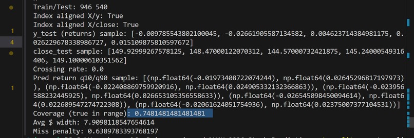
4️⃣ Evaluation
After training, we evaluated on unseen test data using:
Coverage [ \text{Coverage} = \frac{1}{N} \sum \mathbf{1}{ y_{t+1} \in [\hat{y}{low}, \hat{y}{high}] } ]
Average Interval Width
Miss Penalty (distance outside the band)
Since we predict Q10 and Q90, ideal coverage is:
[ \approx 80\% ]
This tests whether our probabilistic forecasts are calibrated.
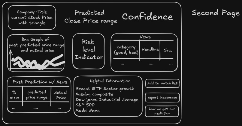
5️⃣ Deployment
We serialized both models into a single .joblib bundle and built an interactive Streamlit dashboard that:
- Displays predicted price range
- Colors bounds relative to current price
- Shows historical prediction bands vs actual
- Computes confidence from interval width
- Visualizes risk via volatility
The system moves from:
Offline training → Model serialization → Real-time inference
📊 What We Learned
1️⃣ Predicting uncertainty is harder than predicting direction
Forecasting the distribution of returns requires modeling volatility regimes and tail behavior.
2️⃣ Coverage ≠ Accuracy
Optimizing quantile loss does not directly optimize coverage. Calibration and generalization matter.
3️⃣ Financial data is heteroskedastic
Volatility clusters. Incorporating rolling and EWMA volatility features significantly improved interval realism.
4️⃣ Data leakage is subtle
Shifting news features correctly was critical. One-day leakage dramatically inflates results.
5️⃣ Simplicity scales
Two LightGBM quantile models performed surprisingly well without deep neural networks.
⚠️ Challenges We Faced
1️⃣ Quantile Undercoverage
Initially, our 80% interval only covered ~60% of outcomes.
This taught us about:
- Regime shifts
- Overfitting
- Tail underestimation
We improved this by:
- Switching to log-returns
- Adding volatility regime features
- Using early stopping
2️⃣ Quantile Crossing
Since Q10 and Q90 are trained independently, predictions can cross.
We handled this by enforcing:
[ \hat{Q}{low} = \min(r{10}, r_{90}) ] [ \hat{Q}{high} = \max(r{10}, r_{90}) ]
3️⃣ Aligning Predictions Correctly
Because our target is next-day return:
Prediction at time ( t ) corresponds to actual close at ( t+1 ).
Ensuring correct temporal alignment was critical for evaluation and dashboard visualization.
4️⃣ UI Consistency
Moving from a single regression model to quantile models required reworking:
- Confidence logic
- Historical band visualization
- Color encoding logic
🌎 Impact
Most retail tools provide deterministic predictions.
Our project provides:
- Uncertainty-aware forecasting
- Interpretable risk bands
- Real probabilistic modeling
- Transparent evaluation metrics
We believe probabilistic forecasting is a more honest way to communicate market uncertainty.
🔮 Future Improvements
- Joint multi-quantile training to reduce crossing
- Distributional boosting (e.g., NGBoost)
- Regime-switching volatility models
- Cross-asset training
- Real-time event risk adjustment
🧩 Final Thoughts
Markets are uncertain by nature.
Our goal was not to predict the future perfectly —
but to quantify the uncertainty of tomorrow.
By combining:
- Machine Learning
- Quantile Regression
- Time Series Modeling
- NLP-based Sentiment Analysis
- Interactive Visualization
we built a system that reflects how real-world risk works:
[ \text{Not a point. A distribution.} ]
Glimpse
Probabilistic. Transparent. Data-driven.
Built With
- data-visualization
- feature-engineering
- finnhub-api
- gradient-boosting
- joblib-(model-serialization)
- lightgbm
- log-return-modeling
- machine-learning
- natural-language-processing-(nlp)
- numpy
- pandas
- parquet-data-storage
- probabilistic-forecasting
- python
- quantile-regression
- scikit-learn-api-(lightgbm-wrapper)
- streamlit
- time-series-forecasting
- vader-sentiment-analysis
- volatility-modeling
- yfinance


Log in or sign up for Devpost to join the conversation.