-
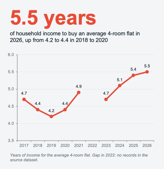
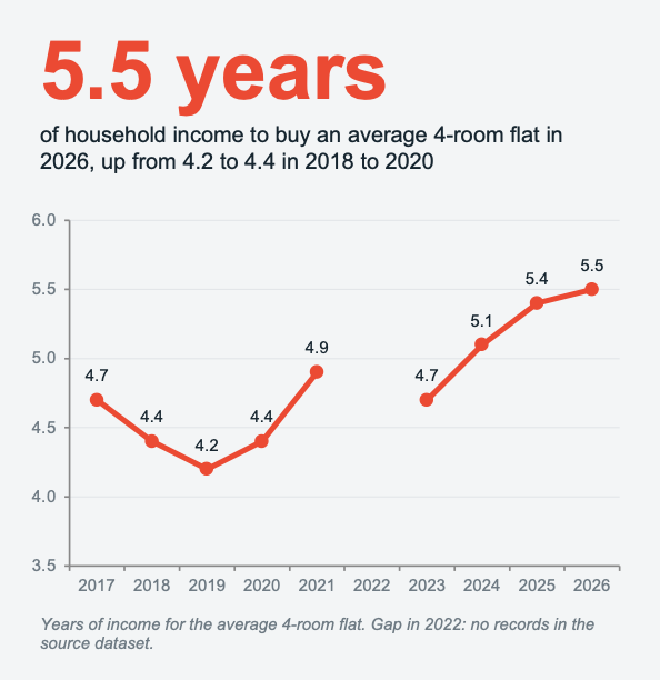
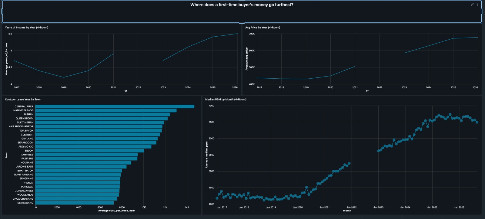
Years of household income for an average 4-room flat, 2017 to 2026. The 2022 gap is missing from the source data, not estimated in.
-
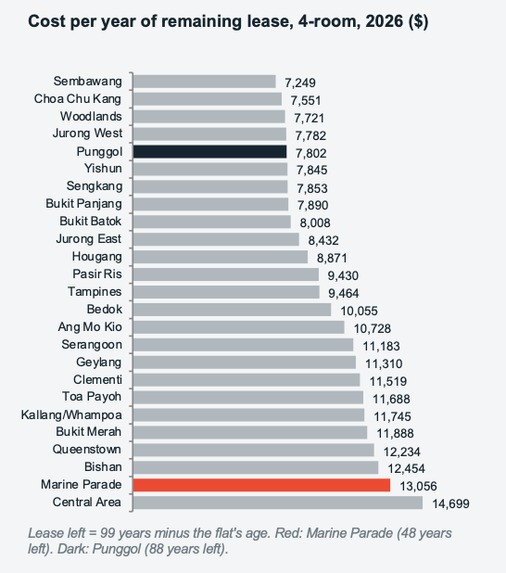
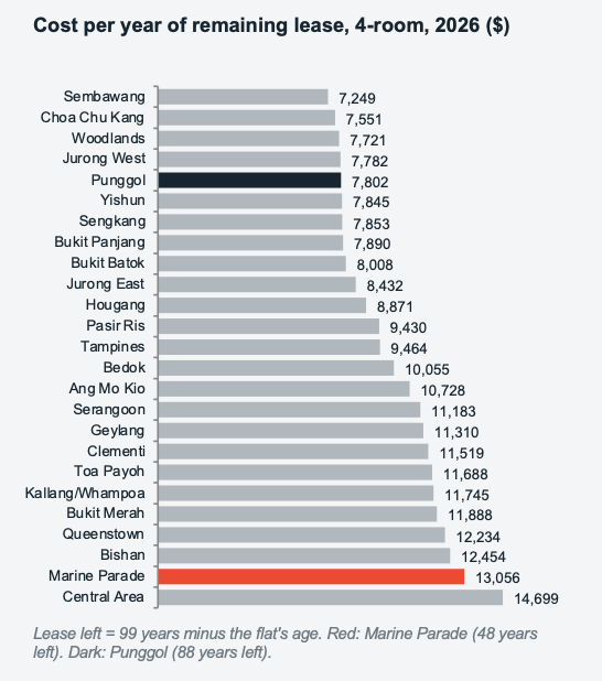
Cost per year of remaining lease, 4-room flats, 2026. Marine Parade (48 years left) costs more per lease-year than Punggol (88 years left).
-
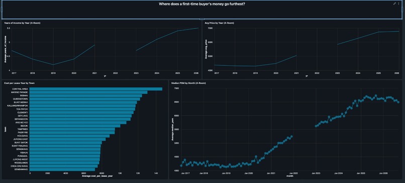
The FlatFair dashboard: affordability trend, town ranking, and monthly price series, built in Databricks SQL and AI/BI.
-
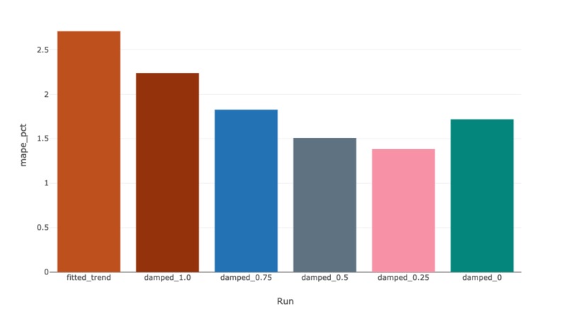
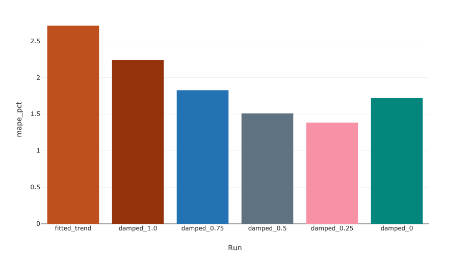
Backtested 6-month forecast error by method. A 25% damped trend (1.38%) beat both a flat baseline (1.72%) and the full trend (2.71%).
-
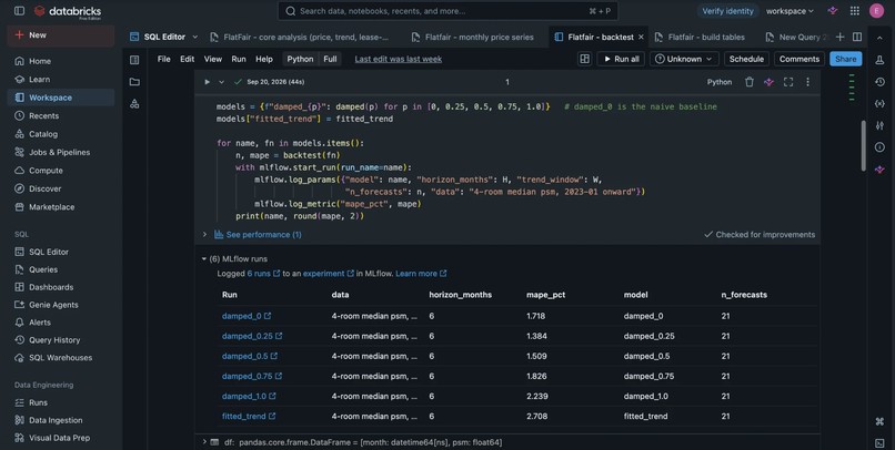
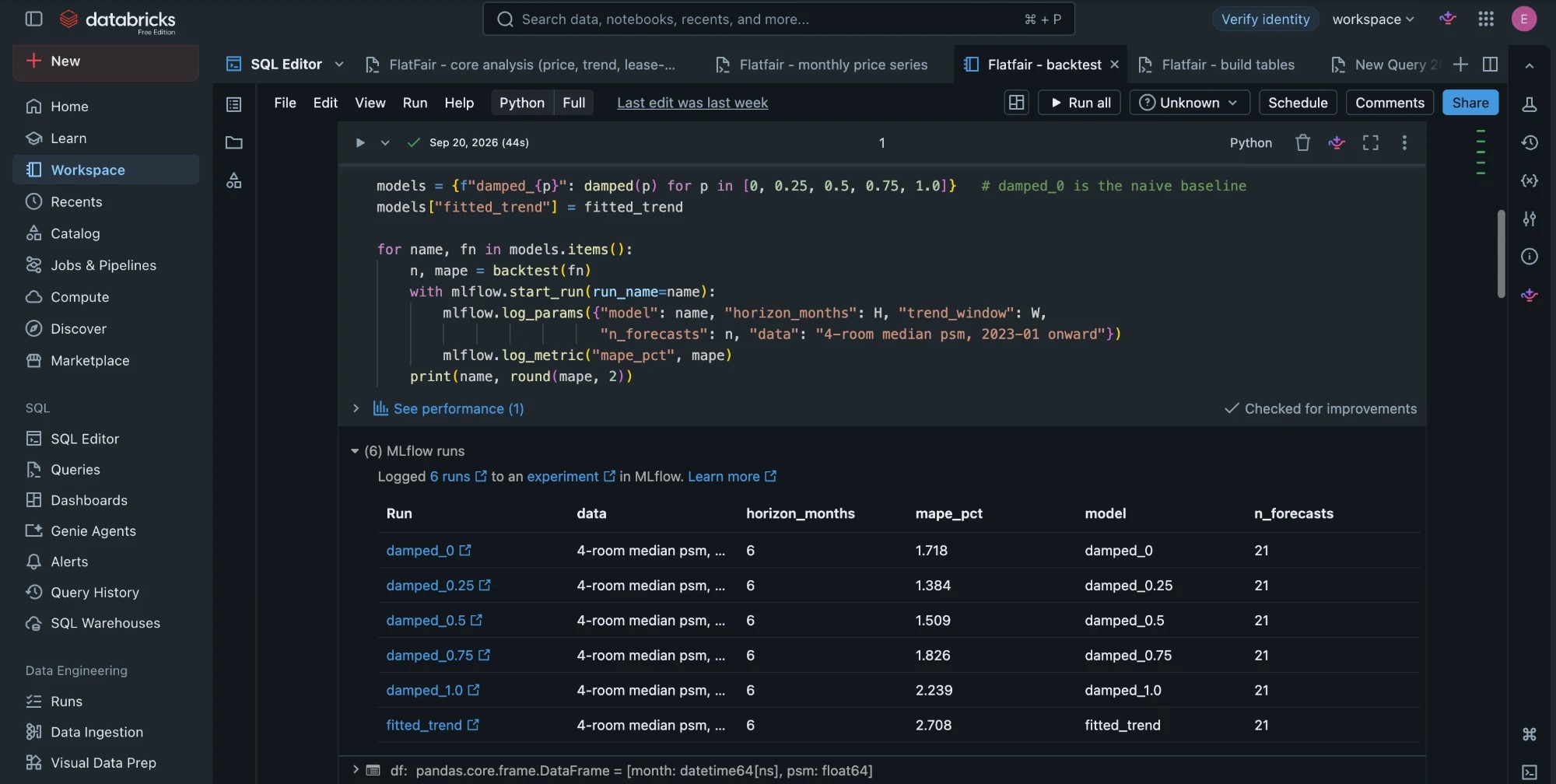
The notebook cell that runs the 6-month backtest and logs each model's parameters and error to MLflow.
-
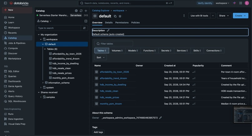
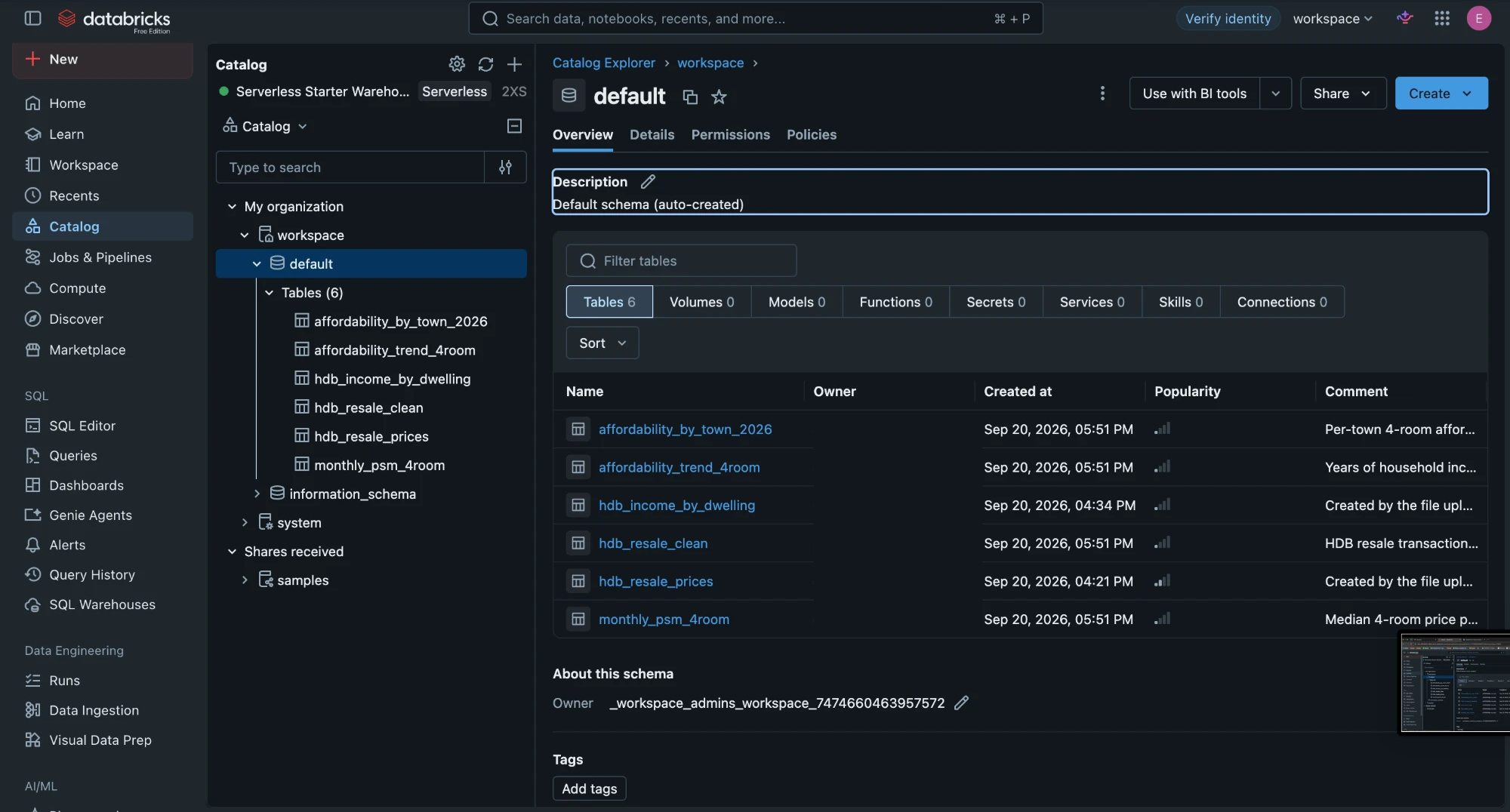
The six Delta tables built from the two source datasets, with descriptions in Unity Catalog.
-
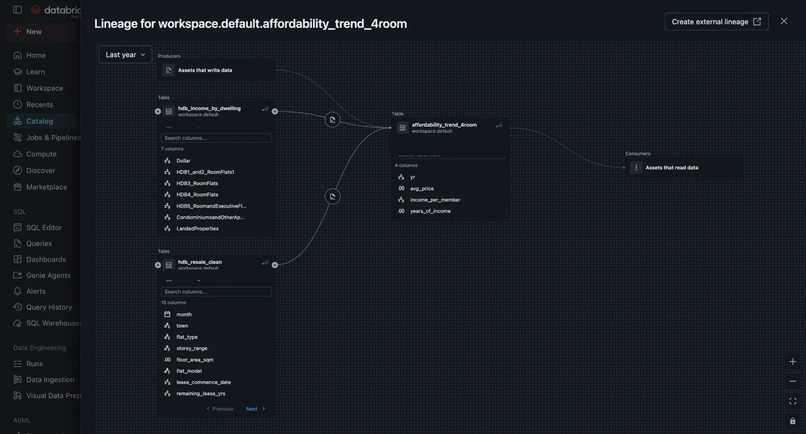
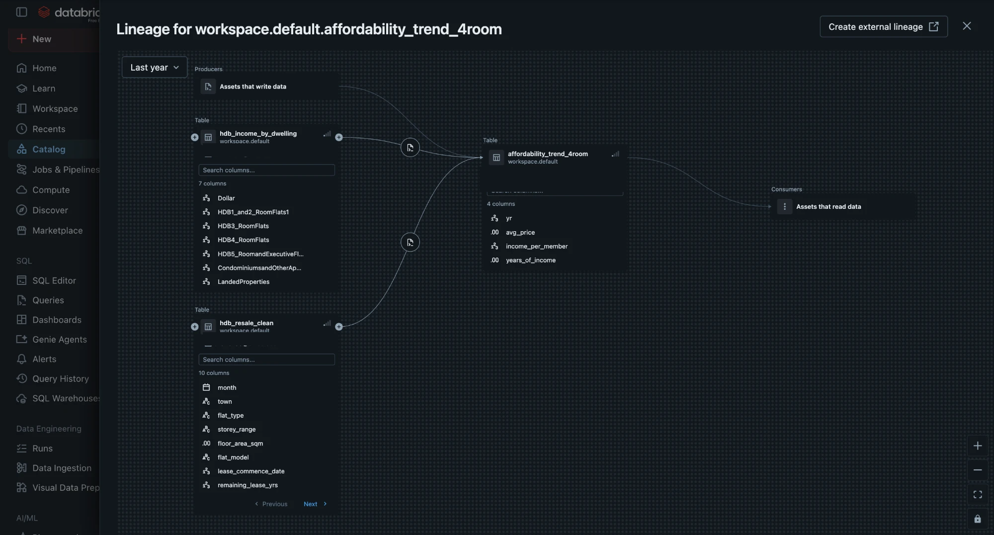
Unity Catalog lineage for affordability_trend_4room, tracing back to the cleaned resale table and the SingStat income table.
Inspiration
Reading through the Round 1 problem statements, I found that several became difficult to pursue after examining the available data. One track's elderly-population data only contained town-level figures from a 2018 survey, while another was supported by a dataset with just four rows. In contrast, HDB's resale dataset contained over 214,000 clean transactions in a single CSV, updated to September 2026, which led me to choose this track.
Exploring the data, I was struck by how many years of household income a 4-room flat now costs, and by how far this had moved since 2020. Rising HDB prices are familiar, but I had not seen affordability expressed as a share of a household's working life. Looking at prices alone also has another limitation, since a flat that appears cheaper may have considerably less of its lease remaining. This led me to build FlatFair around the question of how affordable HDB flats are once both income and remaining lease are considered.
What it does
- Measures a flat's cost in years of household income. The average 4-room flat now costs approximately 5.5 years of household income, compared with about 4.2 to 4.4 years between 2018 and 2020. Across towns, the figure ranges from 4.4 years in Jurong West to 8.4 years in Central Area.
- Adjusts prices for the remaining lease. FlatFair calculates price per year of lease remaining. A flat in Marine Parade costs approximately $13,100 for every lease-year left, compared with about $7,800 in Punggol. Once its remaining lease is counted, a cheaper-looking flat can turn out to be worse value.
- Provides a 6-month national price outlook. I backtested the forecast against a baseline that assumes prices remain unchanged. Nationally, the model achieved an average error of 1.38%, compared with 1.72% for the baseline. At the town level I could not establish a similarly reliable advantage, so FlatFair provides a national forecast range and makes no town-level predictions.
How I built it
I built the project entirely using Databricks Free Edition. I began with two data.gov.sg datasets: HDB resale transactions from January 2017 onwards and SingStat household income by dwelling type. I loaded both into Unity Catalog as managed Delta tables. The upload process remains manual for now because of limitations I encountered during ingestion, and automating this is the first improvement I intend to make.
From there, I used Databricks SQL to construct a cleaned base table. I checked all 214,087 observations for null values, invalid prices and invalid lease dates, without finding any. I then constructed three derived tables covering the affordability trend, town-level lease-adjusted rankings and monthly price series.
Finally, I used a serverless Python notebook to conduct a rolling 6-month backtest across several trend specifications, logging the parameters and resulting errors of each run through MLflow. An AI/BI dashboard built from the same tables displays the affordability trend, town rankings and price series.
Challenges I ran into
The first issue I encountered was that the resale dataset had no transactions for 2022. Before assuming I had made an error during data processing, I queried the live data.gov.sg API and found that a June 2022 query also returned zero records. Given that 2022 coincided with substantial movements in resale prices, estimating the missing observations could have distorted the trend. I therefore excluded the year and explicitly marked the gap on every chart using the affected series.
Ingestion presented another obstacle. Free Edition's serverless compute could not resolve data.gov.sg without identity verification, while direct calls from outside Databricks encountered a network-policy block. Consequently, for Round 1 I uploaded both CSVs manually through the Catalog UI.
I also discovered that town-level forecasting was considerably noisier than the national results initially suggested. Although the damped-trend model outperformed the flat baseline nationally, it won in only 14 of 22 towns. Investigating this further, I found that Clementi's monthly price per sqm can fluctuate by over 40%, largely because relatively few units are resold in some months. Each observation can therefore depend heavily on the particular mix of flats that happened to transact. This prompted me to consider a mix-adjusted index as the next step in improving the model.
Accomplishments I'm proud of
I am particularly pleased that I identified both the 2022 data gap and the Clementi volatility before either could silently distort my conclusions. The forecast also comes with a validated result, a national backtested error of 1.38% compared with 1.72% for the flat baseline.
In an earlier version I tried to incorporate a third dataset, but I could never verify that it existed. Removing it narrowed the project to two datasets and a single question, producing an analysis I could defend.
What I learned
I expected the full trend-following model to perform relatively well, yet it produced an average error of 2.71%, substantially worse than the 1.72% achieved by assuming that prices would not move. Prices had remained relatively flat for over a year, while the model continued extending the earlier upward trend and consequently overshot repeatedly. I found that, for this market and period, a small and damped adjustment towards the trend performed better than either blindly following it or ignoring it altogether.
What's next
- Develop a mix-adjusted price index, preventing months with unusual combinations of large or small flats from distorting the underlying trend.
- Build a buyer-facing tool where users enter their household income and desired flat type and receive the towns that fit their budget, together with each town's lease-value ranking.
- Register the backtested model in MLflow and schedule it to refresh as HDB releases new transaction data.
- If time permits, examine whether flats near newly opened MRT stations experience different price movements from otherwise comparable areas.
