-
-
Final Poster
-

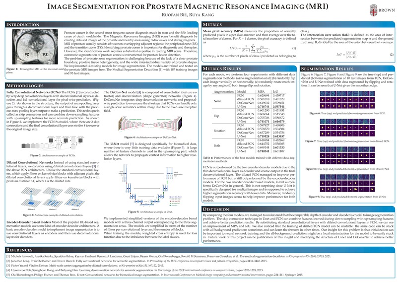
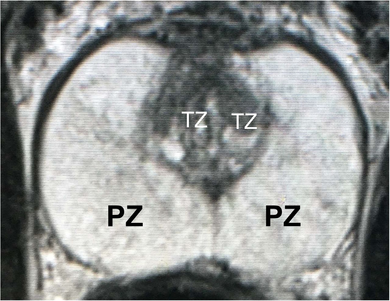
Figure 1: T2-weighted MRI at the maximal axial plane.
-
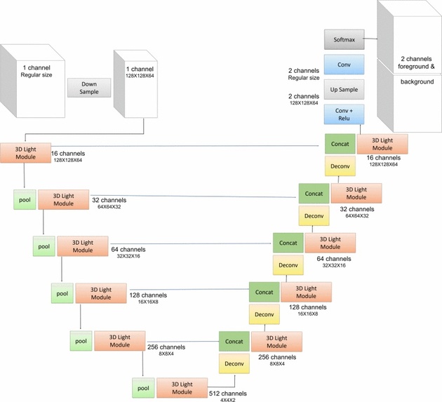
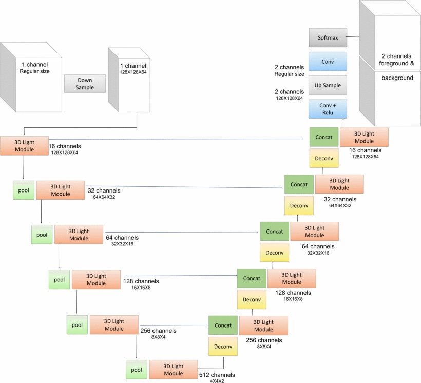
Figure 2: Macro structure network of VnL.
-
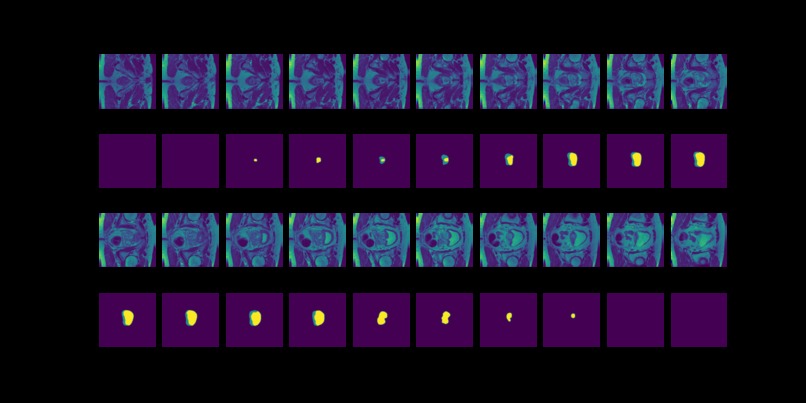
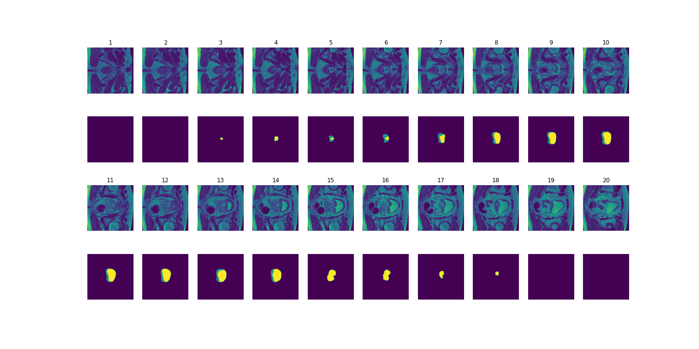
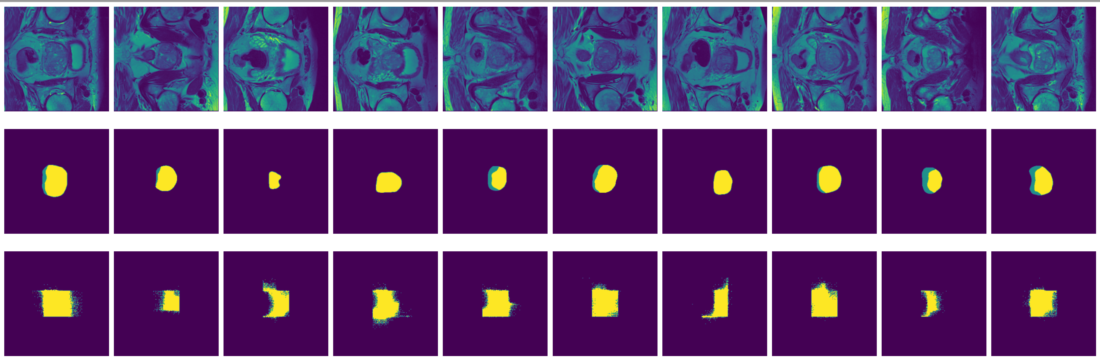
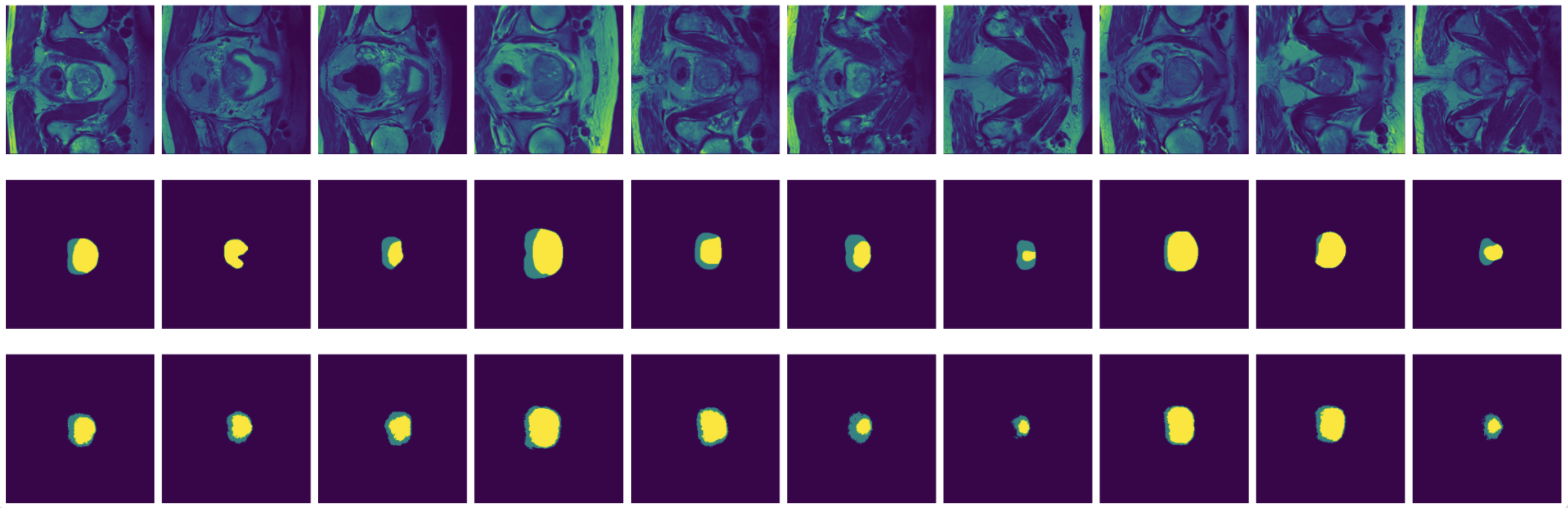
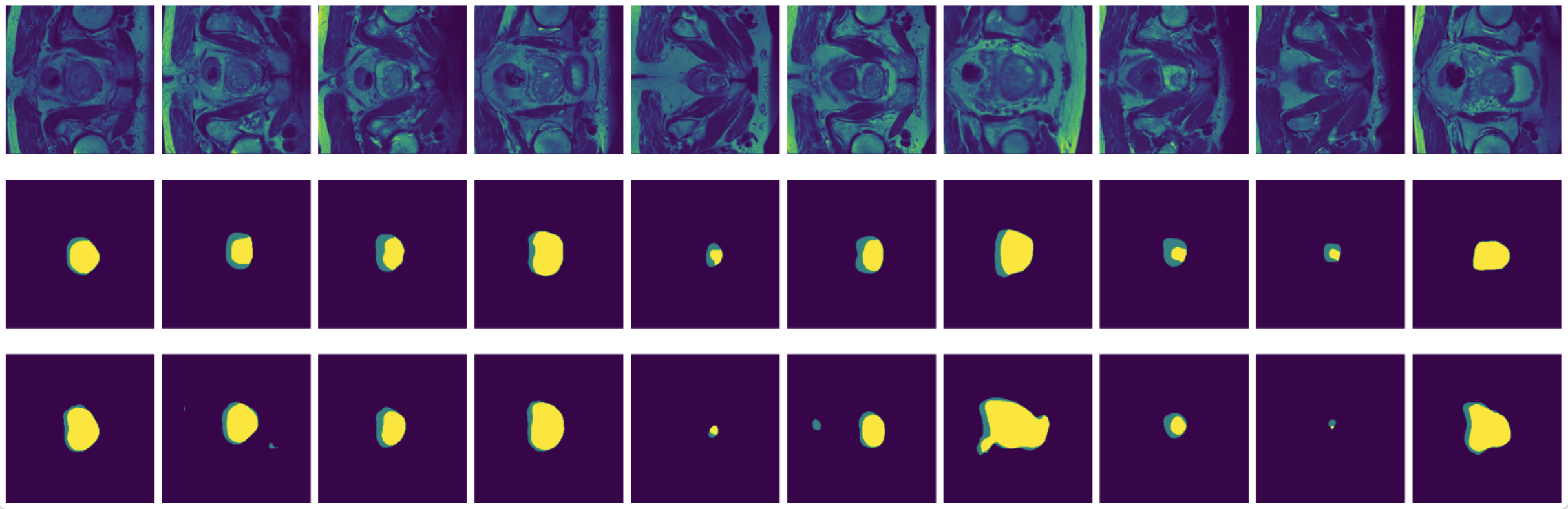
Figure 3: MRI slices (first and thrid rows) from one study with labels (second and fourth rows).
-
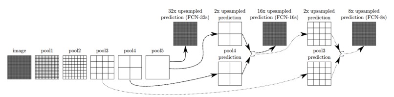
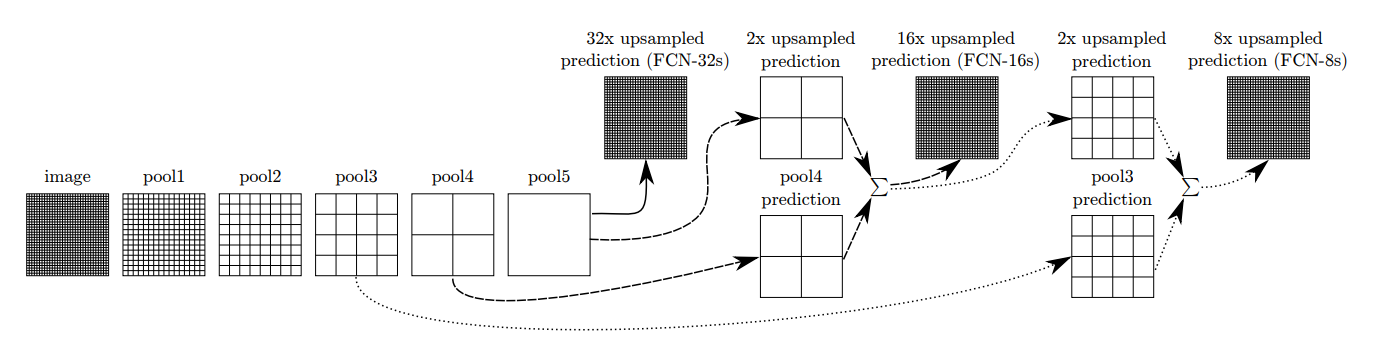
Figure 4: Architecture example of Fully Convolutional Networks.
-
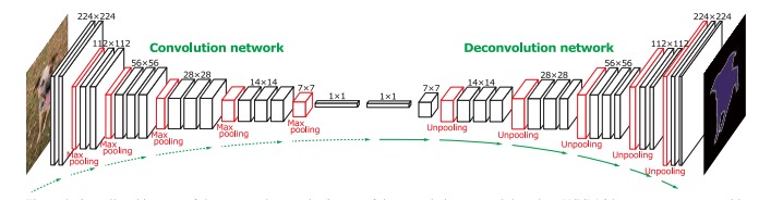
Figure 5: Architecture example of DeConvNet.
-
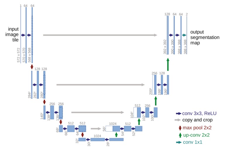
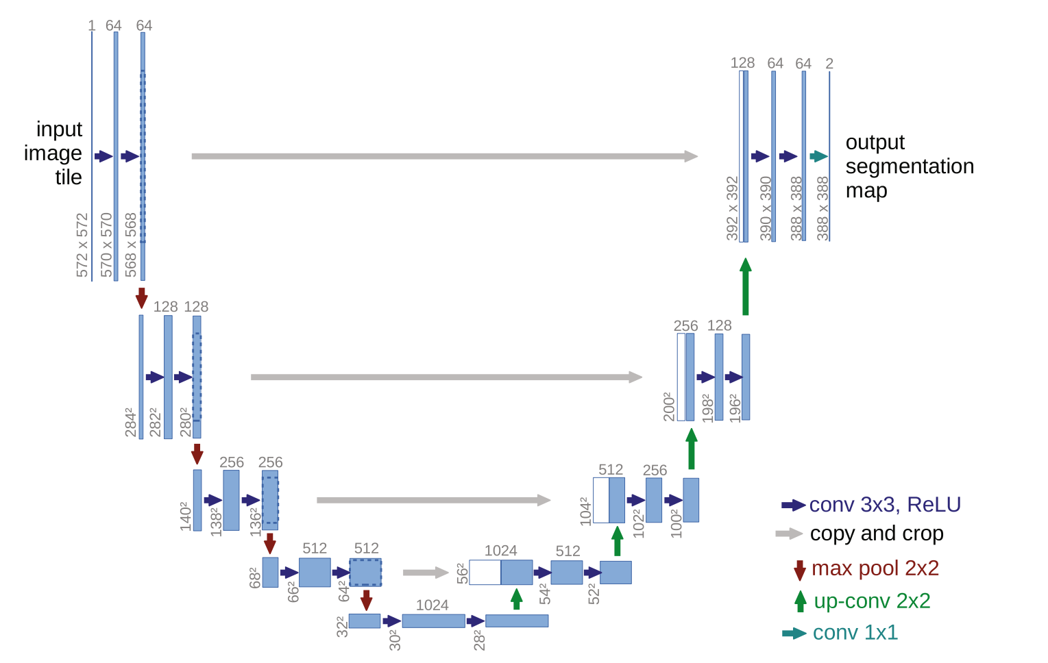
Figure 6: Architecture example of U-Net.
-
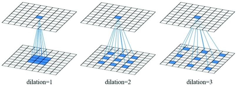
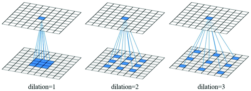
Figure 7: Architecture example of Dilated Convolutional Layer
-
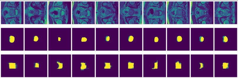
Figure 8: True (top) and predicted (bottom) segmentation from FCN trained with data augmented by flipping and rotation.
-
Figure 9: True (top) and predicted (bottom) segmentation from dilated FCN trained with data augmented by flipping and rotation.
-
Figure 10: True (top) and predicted (bottom) segmentation from DeConvNet trained with data augmented by flipping and rotation.
-
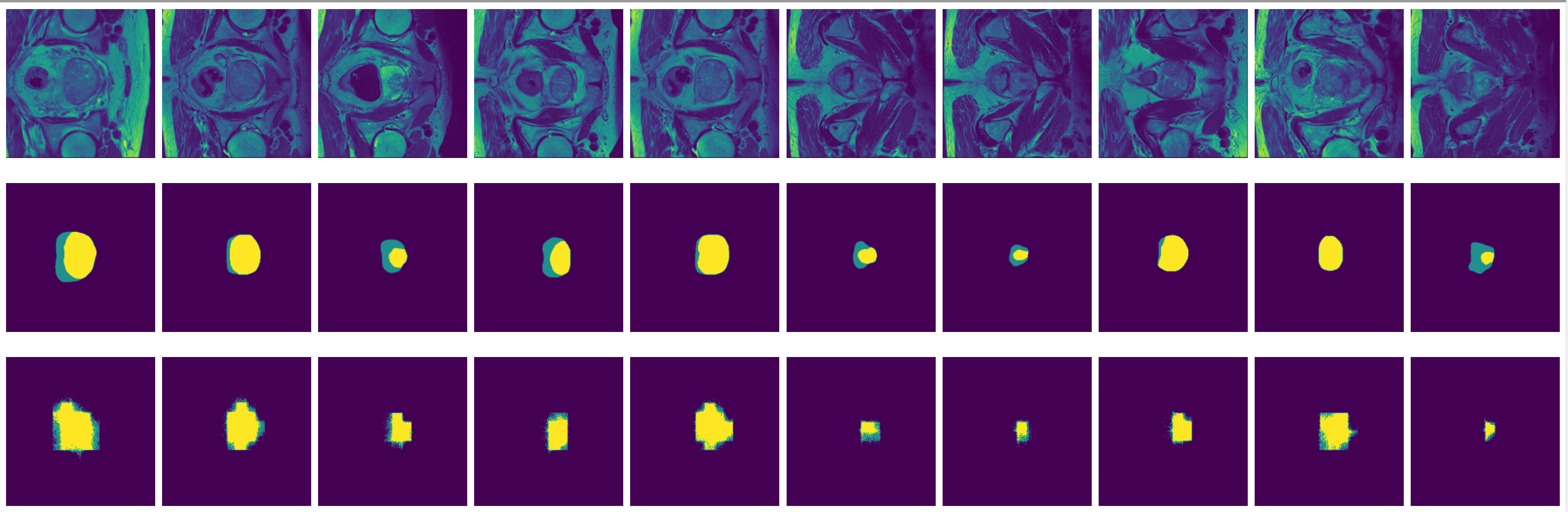
Figure 11: True (top) and predicted (bottom) segmentation from U-Net trainedwith data augmented by flipping and rotation.

FinalProject2470
Ruofan Bie and Ruya Kang
Introduction
In this project, we intend to perform image segmentation with prostate Magnetic Resonance Imaging (MRI) data.
Prostate cancer is the second most frequent cancer diagnosis made in men and the fifth leading cause of death worldwide. [1] A few techniques are used for early detection of prostate cancer, including blood tests, biopsy and imaging tests. The Magnetic Resonance Imaging (MRI) scans create detailed images of soft tissues in the body using radio waves and strong magnets. MRI scans can give doctors a very clear picture of the prostate and nearby areas. [2]
MRI of prostate cancer usually consists of two non-overlapping adjacent regions: the peripheral zone (PZ) and the transition zone (TZ). An example of prostate MRI with labelled zones is shown in Figure 1. Identifying prostate zones is important for diagnostic and therapies. However, the identification work requires substantial expertise in reading MRI scans. Therefore, automatic segmentation of prostate zones is instrumental for prostate lesion detection.

The problem of prostate zone segmentation is challenging because of the lack of a clear prostate boundary, prostate tissue heterogeneity, and the wide inter-individual variety of prostate shapes. [3] In this project, we will be implementing some existing CNN and RNN models for image segmentation using prostate MRI data. We will use a survey for image segmentation using deep learning [4] as a guide, implement selected models and compare their performance.
Related Work
Prior Work
There are some works done for segmenting prostate MRI images using deep learning.
[5] focus on the work done using fully convolutional neural networks (FCNN). They suggested eight different FCNNs-based deep 2D network structures for automatic MRI prostate segmentation by analysing various structures of shortcut connections together with the size of a deep network using the PROMISE12 dataset [6].
[7] mentions that 3D neural networks have strong potential for prostate MRI segmentation. However, substantial computational resources are required due to the large number of trainable parameters. They proposed a network architecture called V-net Light (VnL), which is based on an efficient 3D Module called 3D Light, that minimises the number of network parameters while maintaining state-of-art segmentation results. The proposed architecture replaces regular 3D convolutions of the V-net architecture [8] with novel 3D Light modules. Figure 2 shows the architecture of VnL. The original V-net model consists of encoder and decoder paths with convolutional layers. To reduce the number of parameters, [7] inserts pooling layers between the encoder stages. The novel 3D-Light Module is used in each stage of the encoder and decoder. The 3D-Light Module is a parameter-efficient 3D convolutional block consisting of parallel convolution blocks, blocks composed of regular convolutions, followed by a group convolution. It reduces the number of parameters by 88%−92% in comparison to V-net. The VnL achieves comparable results to V-Net on the PROMISE12 dataset [6] while requiring 90% fewer learning parameters, 90% less hard-disk storage and just 3.3% of the FLOPs.

[9] proposed a transfer learning method based on deep neural networks for prostate MRI segmentation. They also designed a multi-level edge attention module using wavelet decomposition to overcome the difficulty of ambiguous boundaries in the task.
Public Implementation
Some of the model architectures we would like to implement have publicly available implementation.
- FCN-8s: https://github.com/MarvinTeichmann/tensorflow-fcn/blob/master/fcn8_vgg.py
- DeconvNet: https://github.com/HyeonwooNoh/DeconvNet/blob/master/model/DeconvNet/DeconvNet_inference_deploy.prototxt (Caffe)
- U-Net: https://github.com/milesial/Pytorch-UNet/tree/master/unet (Pytorch).
Data
We use a set of prostate MRI data from The Medical Segmentation Decathlon -- a biomedical image analysis challenge. The Decathlon challenge made ten data sets available online. All data sets have been released with a permissive copyright license (CC-BY-SA 4.0), thus allowing for data sharing, redistribution, and commercial usage. [10]
According to [10], all images were de-identified and reformatted to the Neuroimaging Informatics Technology Initiative (NIfTI) format (https://nifti.nimh.nih.gov). All images were transposed (without resampling) to the most approximate right-anterior-superior coordinate frame, ensuring the data matrix x−y−z direction was consistent. Lastly, non-quantitative modalities (e.g., MRI) were robust min-max scaled to the same range. For each segmentation task, a pixel-level label annotation was provided.
The Decathlon challenge provides users with training sets (images and labels) and test sets (images without labels). To evaluate the performance with true labels, we only use the training set provided and randomly select a third of the data to be our own test set.
The prostate data set was acquired at Radboud University Medical Center, Nijmegen Medical Centre, Nijmegen, The Netherlands. It consists of 48 prostate multiparametric MRI (mpMRI) studies, 32 of them have corresponding region-of-interest (ROI) targets (background= 0, TZ= 1 and PZ= 2). Each study contains approximately 15 to 20 slices of MRI images, resulting in 602 images in total. Figure 3 shows the 20 slices from one study. The first and last few MRI slices contain little segmentation information. Therefore, to simplify the problem, we will discard the first and last 5 MRI slices from each study. We will use 10 studies (95 images) as the test set and the remaining 22 studies (187 images) as the training set.
 from one study with labels (second and fourth rows).")
Methodology
Fully Convolutional Networks (FCNs)
The FCNs [11] is constructed by very deep convolutional layers with deconvolutional layers as decoders and 1x1 convolutional layer for pixel-wise prediction. (Figure 4). As shown in the structure, the output of max-pooling layer goes through a deconvolutional layer and then fuse with the previous max-pooling layer output to make a prediction. This technique is called as skip connection and can combine down-sampling features with up-sampling features for more accurate prediction. As shown in Figure 2, we implement the FCN-8s model, where there are 2 skip connections and the final convolutional layer uses strides 8 to recover the original image size.

Encoder-Decoder Based Models
Most of the popular DL-based segmentation models use some kind of encoder-decoder architecture. A basic encoder-decoder model to implement image segmentation is to use convolutional layers as encoders and then use deconvolutional or convolution-transpose layers for decoders. We will implement two of them: DeConvNet for general image segmentation and U-Net for medical image segmentation.
DeConvNet
The DeConvNet [13] is designed on top of the convolutional layers adopted from the VGG 16-layer net [12]. As shown in Figure 5, DeConvNet is composed of convolution and deconvolution networks, where the convolution network acts as the feature extractor and the deconvolution network is a shape generator. The proposed architecture aims to overcome two limitations of FCNs. First, using FCN models, label prediction is done with only local information for large objects. Also, FCNs often ignore small objects and classify them as background. Second, in FCN, the input to the deconvolutional layer is too coarse and the deconvolution procedure is overly simple.

We simplify our DeConvNet model by reducing the number of filters per convolutional layer and incorporating less (de)convolutional blocks. There are no unpooling layers defined in TensorFlow. We make use of the implementation from https://github.com/aizawan/segnet/blob/master/ops.py.
U-Net
The U-Net model [14] is built upon [11]. It is designed specifically for biomedical data, where there is very little training data available. Different from [11], a large number of feature channels is used in the upsampling part. The modification allows the network to propagate context information to higher resolution layers. The network does not have any fully connected layers and only uses the valid part of each convolution. We will implement the simplified version of U-Net model shown in Figure 6 with a three-channel output corresponding to the three segmentation areas. The model is simplified in terms of the number of filters per convolutional layer and the number of blocks.

Dilated Convolutional Models
Due to the translation-invariant property of the convolutional layer, the FCN model is reliable in predicting the presence and roughly the position of objects in an image. However, as a trade-off between classification accuracy and localization accuracy, the FCN model might not be able to sketch the exact outline of the object. Instead of using standard convolutional layers, we consider using dilated convolutional layers [15] in the above FCN architecture. Unlike the standard convolutional layers, which apply filters on kernel-size blocks with adjacent pixels, the dilated convolutional layers apply filters on kernel-size blocks with pixels in distance l-1, where l is the dilated rate (Figure 7).

Since we only have 187 images, we firstly use data augmentation to add rotated or flipped images into the original training set to increase the training sample size and also increase the robustness of our model. All four models are trained with 50 epochs through the whole training set with batch size 1. The trained models are then applied to the test set and compute the accuracy metrics describes below.
Metrics
The model performance for image segmentation is measured differently from for classification. We will evaluate the model using a few new metrics. [4]
Pixel Accuracy
Pixel accuracy (PA) measures the proportion of correctly classified pixels. For K+1 classes, the pixel accuracy is defined as
,
where is the number of pixels of class predicted as belonging to class j.
Mean pixel accuracy (MPA) extends PA to the proportion of correctly predicted pixels in a per-class manner, and then average over the total number of classes.
Intersection over Union
Pixel accuracy has limitations such that it has a bias in the presence of very imbalanced classes, while mean pixel accuracy is not suitable for data with a strong background class. Another segmentation evaluation metric is the intersection over union (IoU). It is defined as the area of intersection between the predicted segmentation map A and the ground truth map B, divided by the area of the union between the two maps:
.
The mean intersection over union (Mean-IoU) is defined as the average IoU over all classes.
In this project, we would expect an accuracy of 50% for all models using the intersection over union metric as a baseline. Our goal is to implement 70-75% of accuracy for the four models. If these accuracies are easily achieved, we would consider adjusting the model to achieve around 90% accuracy.
Results
For each mode, we perform four experiments with different data augmentation methods: (a) no augmentation at all; (b) randomly flip each image vertically or horizontally; (c) randomly rotate reach image by any angle; (d) both image flip and rotation.
| Model | Pixel Accuracy (PA) | Mean Pixel Accuracy (MPA) | Intersection over Union (IoU) |
|---|---|---|---|
| FCN (no aug) | 0.962719 | 0.620694 | 0.459717 |
| Dilated FCN (no aug) | 0.974142 | 0.581018 | 0.481629 |
| DeConvNet (no aug) | 0.974025 | 0.619032 | 0.509451 |
| U-Net (no aug) | 0.976238 | 0.718744 | 0.597541 |
| --- | --- | --- | --- |
| FCN (flip) | 0.962796 | 0.601290 | 0.451951 |
| Dilated FCN (flip) | 0.977338 | 0.606064 | 0.481629 |
| DeConvNet (flip) | 0.979059 | 0.705706 | 0.515348 |
| U-Net (flip) | 0.978152 | 0.741071 | 0.616579 |
| --- | --- | --- | --- |
| FCN (rotation) | 0.969019 | 0.597827 | 0.468806 |
| Dilated FCN (rotation) | 0.976503 | 0.578570 | 0.504504 |
| DeConvNet (rotation) | 0.977549 | 0.637209 | 0.554754 |
| U-Net (rotation) | 0.979722 | 0.719528 | 0.613457 |
| --- | --- | --- | --- |
| FCN (both) | 0.962796 | 0.601290 | 0.451951 |
| Dilated FCN (both) | 0.972596 | 0.644752 | 0.538985 |
| DeConvNet (both) | 0.980162 | 0.698144 | 0.601530 |
| U-Net (both) | 0.973854 | 0.740341 | 0.601107 |
It can be seen that for our task, where the class labels are highly unbalanced, the pixel accuracy is not representative. Therefore, we compare the performance using the mean pixel accuracy over classes and the IoU.
FCN is outperformed by the two encoder-decoder models due to the thin deconvolutional layer as decoder and coarse output in the final deconvolutional layer. The dilated FCN managed to improve performance of FCN but is still outperformed by the encoder-decoder models. For the two encoder-decoder based models, U-Net outperforms DeConvNet in general. This is not surprising since U-Net is specifically designed for medical images and is supposed to achieve higher segmentation accuracy with fewer data. Moreover, randomly flipping input images seems to help improve performance for both of the models. Figure 8 and Figure 9 are the true (top) and predicted (bottom) segmentation of 10 test images from FCN and dilated FCN trained with data augmented by flipping and rotation. Figure 10 and Figure 11 are the true (top) and predicted (bottom) segmentation of 10 test images from DeConvNet and U-Net trained with data augmented by flipping and rotation. It can be seen that U-Net gives a smoother edge than FCN, dilated FCN and DeConvNet.


Ethics
Magnetic resonance imaging (MRI) is a medical imaging technique that uses a magnetic field and computer-generated radio waves to create detailed images of the organs and tissues in a patients' body. It's also an important tool for doctors to detect any abnormalities of the tissue or organ. Developing an image segmentation neural network that can reach high accuracy of detecting prostate can help to relieve doctors' burden in manually checking the MRI and can increase efficiency in the medical system. However, developing such neural networks doesn't necessarily mean physicians never have to look at MRI. The neural network results would justify the physician's diagnosis to secure the diagnosis process.
Challenges
One challenge of MRI segmentation is the imbalance between labels. Since the cross-entropy loss function is based on pixel-wise accuracy, it’s easy for our models to produce all-background predictions. To solve this problem, we down-sampled all-background images in the training set and used weighted cross-entropy as loss function. Specifically, we assign weight ratio 1:3:3 to label 0, 1 and 2. After this adjustment, it becomes easier for the DeConvNet and U-Net to learn the position and shape of the prostate (IoU accuracies are over 60%). Note that down-sampling results in less training data, so augmentation is necessary for a better performace.
Another challenge is that the original FCN-8s model still failed to learn any feature and kept producing all-background prediction. After comparing the structure of FCN and U-Net, we realize the importance of the comparable depth of encoder and decoder in image segmentation. We also noticed that by using stride 8 in the last deconvolutional layer in the FCN, the output of FCN can be very coarse. After increasing the number of filters and reducing strides in the deconvolutional layers of FCN, we managed to improve the performance of FCN and reached 48.227% accuracy in IoU. Furthermore, we considered using dilated convolutional layers in the FCN model. The dilated convolutional layers apply filters on kernel-size blocks with pixels in l-1 distance, where l is the dilated rate. Since dilated convolutional network might be able to extract information from larger region, the dilated FCN managed to improve the performance (5% improvement in IoU for none augmentation, 14% improvement in IoU for flip augmnetation, 8% improvement in IoU for rotation augmentation and 12% improvement in IoU for both augmentation).
The third challenge is that the two encoder-decoder based models do not learn well in its originally proposed architecture. One possible reason is that the models may be too complicated for this task so they overfitted to the noise. Moreover, the original DeConvNet and U-Net model are too large for a 16GB GPU to train. To solve the problems, we simplified the encoder-decoder models by reducing the number of encoder and decoder blocks as well as reducing the number of filters per block.
Reflection
In this project, we managed to implement our basic goals and part of the target goals: implementing 4 image segmentation model and reach IoU and mean pixel accuracy over 50%. We planned to reproduce the proposed model architectures from the original papers. However, it turned out that simpler models of same structure performed well. Also, we performed more data pre-processing than proposed due to the high imbalance in segmentation labels. Using weighted loss helped training as well.
During the project process, we found the performance of models are poorer than our expectation. There are two possible reasons for this: 1. The training set is relatively small. After down-sampling the all-background images, there are only 187 original images in the training set and 561 images after both flip and rotation augmentation. 2. Unlike ordinary figures where there are three color layers and the area of subjects and background is usually balanced, the MRIs only have one color layer and the position of the prostate is usually at the center of the image and the area of prostate is usually much smaller than the background. This increase the difficulty for neural networks to learn features.
Our project shows that comparable depth of encoder and decoder is crucial to segmentation of such kind of images. Deep convolutional layers are used to extract features from the inputs while deconvolution, upsampling or unpooling layers should be incorporated to reconstruct the inputs moderately (in contrast to FCN, where only a coarse deconvolution layer is applied). Moreover, for many image segmentation tasks where the label classes are highly unbalanced, adjusting the model with appropriate class weights is also very effective. By comparing the FCN and dilated FCN model, we also found that dilated convolutional layers might be better at learning features in this problem.
We also noticed that the training of dilated FCN model can be unstable: the same code can be stuck with all-background predictions sometimes and can learn the features in other times. Our insight for this problem is that initialization can be important to neural network training and the all-background prediction might be a local minimization for the model to be easily stuck with. In our future work, we can explore the reason why dilated FCN failed to learn any feature occasionally and try to modify the structure of DeConvNet and U-Net, such as using dilated convolutional layers, to see whether the performance of the two models can be improved. Existing models with pretrained weights could also be involved in the comparison.
Division of labour
Ruofan is responsible for running the FCN and dilated convolutional models. Ruya is responsible for running the encoder-decoder models. The report and the poster are works of collaboration.
References
[1] Prashanth Rawla. Epidemiology of prostate cancer. World journal of oncology, 10(2):63, 2019. pages 3
[2] American Cancer Society. Cancer Statistics Center. Tests to diagnose and stage prostate cancer. URL http://cancerstatisticscenter.cancer.org [Accessed8thNovember2021]. pages 3
[3] Nader Aldoj, Federico Biavati, Florian Michallek, Sebastian Stober, and Marc Dewey. Automatic prostate and prostate zones segmentation of magnetic resonance images using densenet-like u-net. Scientific reports, 10(1):1–17, 2020. pages 3
[4] Shervin Minaee, Yuri Y Boykov, Fatih Porikli, Antonio J Plaza, Nasser Kehtarnavaz, and Demetri Terzopoulos. Image segmentation using deep learning: A survey. IEEE Transactions on pattern analysis and Machine Intelligence, 2021. pages 3, 8
[5] Tahereh Hassanzadeh, Leonard GC Hamey, and Kevin Ho-Shon. Convolutional neural networks for prostate magnetic resonance image segmentation. IEEE Access, 7:36748–36760, 2019. pages 3
[6] Geert Litjens, Robert Toth, Wendy van de Ven, Caroline Hoeks, Sjoerd Kerkstra, Bram van Gin-neken, Graham Vincent, Gwenael Guillard, Neil Birbeck, Jindang Zhang, Robin Strand, FilipMalmberg, Yangming Ou, Christos Davatzikos, Matthias Kirschner, Florian Jung, Jing Yuan, Wu Qiu, Qinquan Gao, Philip aEddiea Edwards, Bianca Maan, Ferdinand van der Heijden, Soumya Ghose, Jhimli Mitra, Jason Dowling, Dean Barratt, Henkjan Huisman, and Anant Madabhushi. Evaluation of prostate segmentation algorithms for mri: The promise12 challenge. Medical Image Analysis, 18(2):359–373, 2014. ISSN 1361-8415. doi: https://doi.org/10.1016/j.media.2013.12.002. URL https://www.sciencedirect.com/science/article/pii/S1361841513001734. pages 3, 4
[7] Ophir Yaniv, Orith Portnoy, Amit Talmon, Nahum Kiryati, Eli Konen, and Arnaldo Mayer. V-netlight-parameter-efficient 3-d convolutional neural network for prostate mri segmentation. In 2020 IEEE 17th International Symposium on Biomedical Imaging (ISBI), pages 442–445. IEEE, 2020. pages 3
[8] Fausto Milletari, Nassir Navab, and Seyed-Ahmad Ahmadi. V-net: Fully convolutional neural networks for volumetric medical image segmentation. In 2016 fourth international conference on 3D vision (3DV), pages 565–571. IEEE, 2016. pages 3
[9] Xiangxiang Qin. Transfer learning with edge attention for prostate mri segmentation. arXivpreprint arXiv:1912.09847, 2019. pages 4
[10] Michela Antonelli, Annika Reinke, Spyridon Bakas, Keyvan Farahani, Bennett A Landman, GeertLitjens, Bjoern Menze, Olaf Ronneberger, Ronald M Summers, Bram van Ginneken, et al. The medical segmentation decathlon. arXiv preprint arXiv:2106.05735, 2021. pages 4
[11] Jonathan Long, Evan Shelhamer, and Trevor Darrell. Fully convolutional networks for semantic segmentation. In Proceedings of the IEEE conference on computer vision and pattern recognition, pages 3431–3440, 2015. pages 5
[12] Karen Simonyan and Andrew Zisserman. Very deep convolutional networks for large-scale image recognition. arXiv preprint arXiv:1409.1556, 2014. pages 6
[13] Hyeonwoo Noh, Seunghoon Hong, and Bohyung Han. Learning deconvolution network for semantic segmentation. In Proceedings of the IEEE international conference on computer vision, pages 1520–1528, 2015. pages 6
[14] Olaf Ronneberger, Philipp Fischer, and Thomas Brox. U-net: Convolutional networks for biomedical image segmentation. In International Conference on Medical image computing and computer-assisted intervention, pages 234–241. Springer, 2015. pages 6
[15] Liang-Chieh Chen, George Papandreou, Iasonas Kokkinos, Kevin Murphy, and Alan L Yuille. Semantic image segmentation with deep convolutional nets and fully connected crfs. arXivpreprint arXiv:1412.7062, 2014. pages 7
Built With
- python
- tensorflow


Log in or sign up for Devpost to join the conversation.