-
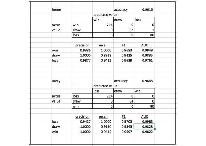
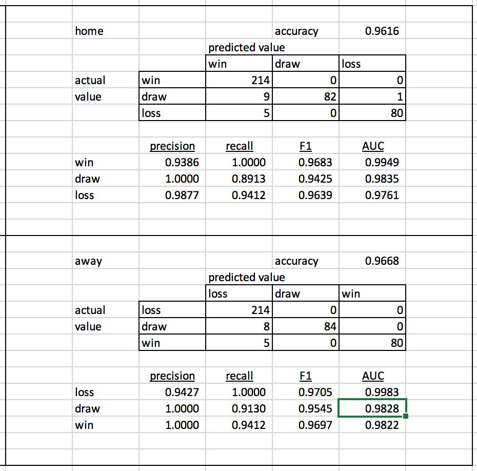
Confusion Matrix
-
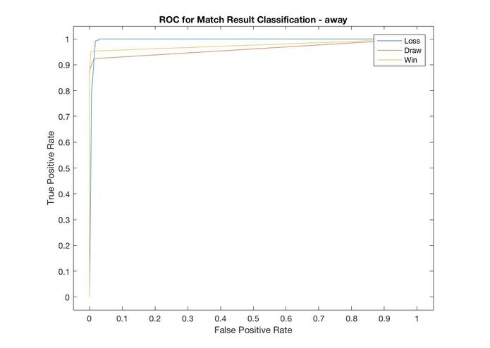
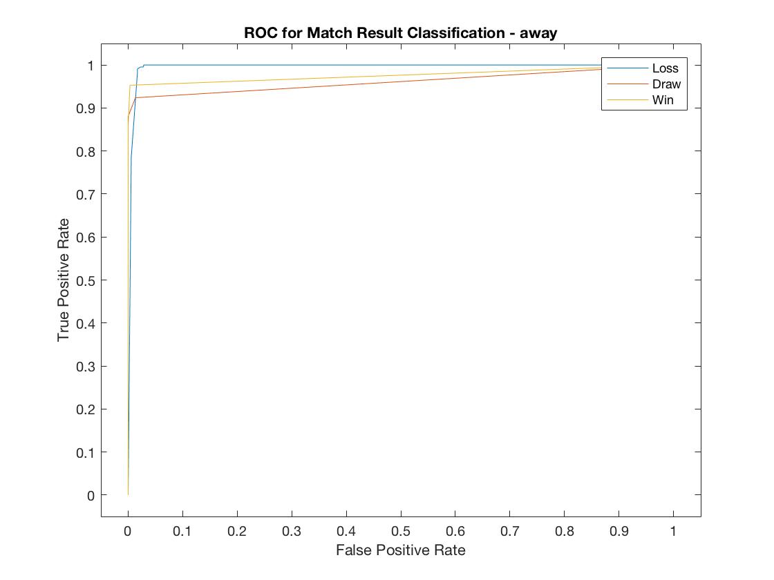
away ROC
-
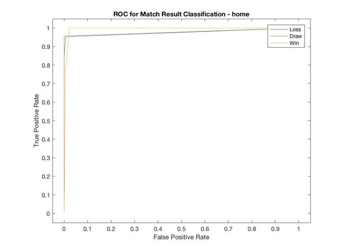
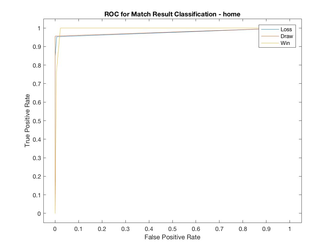
home ROC
The PRETIMOM: Player Relative Evaluation to Influence Match Outcomes Model
A Match Prediction Model Incorporating Speed of Play and Positionally Sorted Player Ratings
Team Dan Reck Yvon Kadeoua Jack Painter Alex Moses Derek Johnson
Problem Definition
Can the Fifa 18 overall player ratings, acting as a proxy for a team’s own scouting information, be utilized to predict outcomes of MLS matchups?
High Level Summary
Our analysis shows that the average FIFA 18 rating of a team’s lineup by player group (backs, central mids, wings, and strikers), the relative strength of player groups within a match (for example, which team has stronger central midfielders), along with a team’s season-long Game Speed metrics yielded accurate match result predictions 97% of the time using Support Vector Machine classification models. The inclusion of the Game Speed metrics reflect how effectively a certain lineup is able to deploy a particular play style. This provided significant improvement over a model using only the FIFA aggregate player rankings of the players on the field for a match and the relative difference in aggregate player rankings in that match, which was only 54% accurate in determining the result.
MLS teams could utilize this back-end analysis to see how changes to their lineup, in combination with the team’s expected speed of play against a particular opponent, to improve their expected outcome in a match. Extending this model to incorporate salary information would help teams determine how best to allocate funds to construct their squads.
Model Creation and Data Cleansing
Game Speed Calculation - (Working R script file) Distance Travelled A function titled ‘distance’ is created, to calculate the distance between 2 (x,y) coordinates. This formula takes inputs of X1, Y1, X2, and Y2, and calculates the square root of [(X2-X1)^2 + (Y2-Y1)^2]. We apply a scaling factor to each of the x and y values, to translate the x,y coordinates into values representative of meters from the endlines. The resulting distance travelled represents the distance the ball travelled in meters.
Time We calculated a new variable which translates the period_min and period_sec variables, into total seconds from game start (this is the ‘cumulative_time’ variable) We then take the difference of the cumulative_time from each row to the next, to calculate the seconds associated with each event (this is the ‘event_seconds’ variable)
Set Possession Start Start of game If team_id changes from the current row to the next, the ‘next’ row will be the start of a new possession Unless, that next event row was an event_type_id of 5, 6, 7, or 44 (Out, Corner Awarded, Tackle, or Aerial). These are events that the Opta data will assign to the opposing team, or duplicate for both teams, and may signal the end of a possession, but not necessarily the beginning of a new one. If the current row event_type_id = 4, 5, or 6 (Foul, Out, or Corner Awarded) and the next row is an event_type_id = 1, then the ‘next’ row will be considered the beginning of a new possession. This signifies a restart.
Set Possession End If event_type_ID = 1, 3, or 4 (pass, take on, foul) has an outcome = 0, this marks the end of a possession. If an event_type_id = 5, 7, 15, 60, or 61 (Out, Tackle, Attempt Saved, Chance Missed, Ball Touch), this marks the end of a possession.
Determine Possession_Life by event This field is built recursively, and relies on previous values to determine the next. The first value in the data set is set to ‘Begin’. If the next row has a possession_end = 1, then this event ends the possession, and sets the Possession_Life variable = ‘End’ If the next row has a possession_start = 1, then the value is set to ‘Begin’ But, if not, and the possession_end = 1, or is also = 0, the Possession_Life variable = ‘n/a’ and will be removed from the dataset eventually. When a possession has started, and before it has ended, this variable will be = ‘Continue’ to represent that the possession is active during this event.
Possession_Life = ‘n/a’ rows are removed from the dataset, since this represents a non-meaningful event from an active possession perspective (ball out of play, or not clearly controlled)
The first row of each possession is calculated, and used as an identifier for a possession. Time and distance_travelled are aggregated by ‘first_row’ to represent the total distance travelled by the ball during the possession, and the total seconds the possession lasted. Some possessions include events for both teams. In these cases, the team with the majority of the time during the possession is selected, while the other team’s data is removed. The result is the ‘df_single_possessions_deduped’ dataframe
Distance_Travelled, and Time are rolled up to the team_id/game_id level. Game speed is calculated as Distance_Travelled / Time.
Player Group Relative Ranking + Game Speed Support Vector Machine to Predict Match Outcome - (Working Matlab script file)
- Players classified as Backs, Central Mids, Wings, and Strikers based on their FIFA club position for the 2017 MLS season. For those marked as SUBS or RESERVE, we utilized TransferMarkt data to assign a position. Keepers were excluded.
- MLS 2017 Match data utilized to determine which players were on the field for every match that season. FIFA ratings averaged for each class of player who played in a given match. This gives us the relative strength of class of players who were on the pitch. This acts as a proxy for team scouting data that a Sporting Director might use in constructing a squad.
- These player class ratings were standardized against the full season to ensure that the range of values don’t skew the model.
- Delta calculated for player class ratings within each given match - ex: difference between home backs and away backs. Gives strength by player class relative to the opponent.
- These deltas were standardized against the full season to ensure that the range of values don’t skew the model.
- Appended Game Speed Calculations. These were season long values for each team. Again, the data was standardized.
- Appended result of the match for each side - 0 for a loss, 1 for a draw, 3 for win. This is used as the target value in the Support Vector Machine.
- Data were split into home data set and away data set to avoid possible interactions with the in-match deltas in step 4.
- Separate Support Vector Machines (SVM) built to predict wins, draws, and losses.
- Simple voting based on predictions from each win, draw, and loss SVM. The model predicting highest probability of a given result wins.
Model Results: The Home model accurately predicted the result (win, draw, or loss) 96.2% of the time. F1 scores, a measure that combines the precision and recall of the model, all exceed .94 and the areas under the ROC curve (AUC) all exceeded .97, suggesting this is a strong model.
Similar results were found in the Away model. It was accurate 96.7% of the time. F1 scores all exceeded .95 and AUC all exceeded .98.
We found significant value in grouping player ratings by position. A model using only the FIFA aggregate player rankings of the players on the field and the relative difference in player rankings within a match was only 54% accurate in determining the result.
Future Considerations to Build Upon and Improve the Product
Model Create sub-models that look at scouting attributes (akin to the FIFA skill rankings) for each position grouping to better understand measures of strength. We would look to answer what composition of skill attributes by position leads to success. These would be used by a Sporting Director to create team specific player strength rankings (instead of these FIFA ranking proxies). Development Academies could build the skill attributes of their own team players into the model instead of the MLS players we used to determine their best starting XI. Incorporate market values and salaries of players into model to provide insight into which players are underrated and where teams can buy the maximum wins. Incorporate internal MLS scouting data (assuming this exists at each club), instead of FIFA 18 data, to represent more up-to-date information. Our analysis shows that using this type of data can be a good predictor. Run analysis on 2016/2017 data, use results to predict 2017/2018 data to validate the predictive accuracy. Weighting minutes played with player ratings, to better reflect the aggregated ratings on the field during the game. Speed of Play Further break down speed of play analysis to position group and individual player. This could produce an independently useful Speed of Play metric for all players. Continue to refine and improve the logic behind the speed of play metric, to improve accuracy. Weighting movement towards the opposition goal as heavier. Update logic to ensure all downtime is removed from the time of possession variable. Other Develop a front-end application that allows for ease of line-up tweaking, to see expected impacts. Can utilize historical speed of play for opposition, with ability to modify.

Log in or sign up for Devpost to join the conversation.