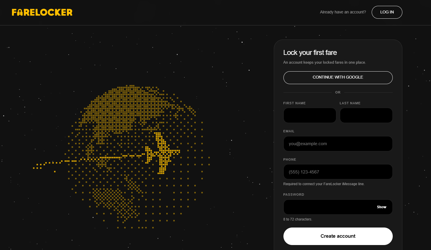
Inspiration

Airline tickets are options in reverse: the carrier can reprice until you buy, and travelers eat the volatility. We kept seeing people “almost book,” watch a fare drop (or jump), and feel stuck—especially when plans weren’t final yet.

FareLocker flips that. Instead of forcing an instant purchase, we sell a short-dated American put on the fare: pay a fee up front, lock a strike, and if the price falls you can exercise for a cash payout. Inspired by how real options desks separate trend from noise, we asked: can we make fare insurance feel like a product a traveler would actually use—from search to iMessage—not just a spreadsheet?

What it does

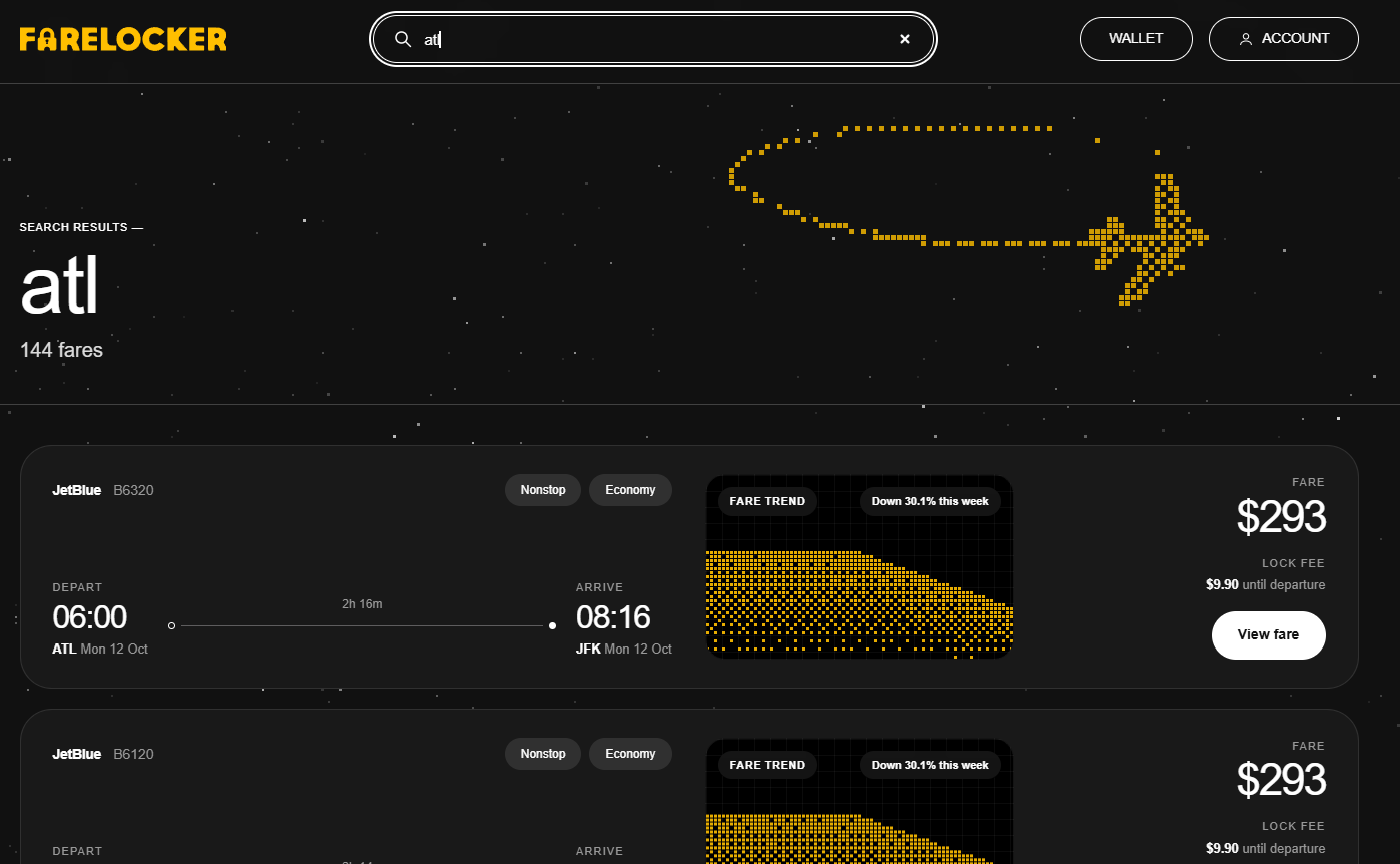
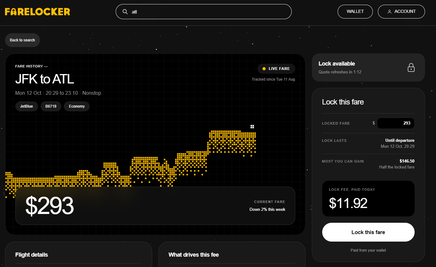
Search real (and demo) flights, see a live FareLock fee next to the fare
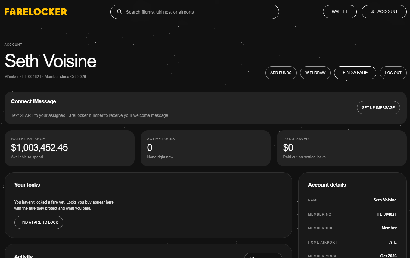
Buy a lock from a wallet balance; fee is charged once at purchase
Mark-to-market and early exercise before departure
Payout is the capped intrinsic put value—fee is not refunded or charged again
Natural-language search / quote paths, plus Photon/iMessage onboarding for a chat-native flow
Simulated XD* flights so we can demo ITM motion without waiting on Google

How we built it

Product model. A FareLock is insurance against a decline. While open, exercise pays:

$$ \mathrm{payout} = \min(\max(K - S, 0),\; 0.5 K) $$

Because exercise is American (any time until departure), we don’t use Black–Scholes. We price with a Cox–Ross–Rubinstein lattice.

Pricing pipeline (backend: FastAPI + Postgres):

Fit a route fare curve so predictable “days-to-departure” drift isn’t treated as vol:

$$ f(d, \mathrm{dow}, \mathrm{hol}) $$

Form the residual:

$$ X = S / f^{\mathrm{flight}} $$

Estimate bucketed volatility with shrinkage to a prior.
Run a CRR American put on that residual, rescale to dollars.
Charge a loaded fee (with a small dollar floor for UX):

$$ \mathrm{fee} = (1+\lambda)\, V^{\mathrm{model}} $$

Product surface. JWT auth, wallet ledger, lock purchase/exercise/settlement jobs, fare search with Google Flights where available, and Spectrum/Photon for iMessage. For the pitch we layered sim flights (deterministic value-noise prices + day-anchored history) so judges can watch a lock go ITM live.

What we learned

Separating term-structure drift from residual vol matters more than fancy vol models when the sell window is only about 30 days
“Smart search” is mostly careful entity extraction (airports, dates, one route)—LLMs are optional; ambiguity handling is mandatory
Demo systems need first-class design: live prices can move, but history charts must not reshuffle every poll
Custom strikes only make sense if the pricer takes spot and strike separately; treating them as ATM silently breaks the economics

Challenges

Sparse / missing curves — real routes need history; demo flights had none, so lock quotes failed until we added a sim pricing fallback
Settlement reality — matching a live fare at exercise/expiry is messy (provider gaps → pending_verification)
Dual channels — website + iMessage (Photon) with shared auth and wallet semantics
Hackathon timeboxing — shipping a coherent story (search → quote → buy → MTM → exercise) beat polishing every edge case

What’s next

Fare volatility isn’t unique to airlines. The same “price moves while you decide” problem shows up on Amtrak, hotels, and other inventory-managed travel. We want FareLocker to become a general travel price-protection layer—put the timing risk back on a priced instrument, and put control back with the traveler. Next up: broaden coverage, harden settlement and payout rails, and keep tightening the curve/vol machinery as we collect more data.

Technical Details

For the curious (and the brave): a deeper look at how we value a FareLock. Skim or skip if you just want the product story above.

FareLocker prices an American put on a flight fare. The traveler pays a fee up front; while the lock is open they may exercise for a capped cash payout. Default strike is the purchase-time fare, though the API also supports a custom strike against spot.

$$ \mathrm{payout} = \min(\max(K - S, 0),\; 0.5 K) $$

Sell window: roughly 30 days or fewer to departure. Because exercise can happen any day before expiry, we use a Cox–Ross–Rubinstein (CRR) binomial lattice rather than a European closed form.

One-sentence model: strip out the predictable fare lifecycle, price an American put on the near-stationary residual, then apply a loading for risk we cannot hedge.

observations
  → route curve f(d, dow, hol)
  → flight premium δ
  → residual X = S / f_flight
  → bucketed σ(X) with shrinkage
  → CRR American put on X (dollarized via f)
  → fee = (1 + λ) · V_model

1. Route term structure

Raw fares trend as departure approaches (yield management). That drift should not be treated as option vol.

For each route we build a cheapest-fare index (min observed price per departure date) and fit on log fare:

$$ \ln S(i) = \alpha + s(d(i)) + \beta^{\mathrm{dow}}(i) + \gamma\cdot\mathrm{holiday}(i) + \varepsilon(i) $$

s(d): step function over days-to-departure buckets (1,3), (4,7), (8,14), (15,21), (22,30), (31,45), (46,60) with (1,3) absorbed into the intercept
day-of-week dummies (Wednesday baseline)
holiday binary flag

Dollar curve:

$$ f(d,\mathrm{dow},\mathrm{hol}) = \exp\bigl(\hat\alpha + \hat s(d) + \hat\beta^{\mathrm{dow}} + \hat\gamma\cdot\mathrm{hol}\bigr) $$

with days-to-departure clamped to the range 1 through 60. Routes with too few index rows keep the previous fit.

2. Flight-level premium

Flights share lifecycle shape but differ in level (banked departure, carrier, etc.):

$$ \delta^{\mathrm{flight}} = \mathrm{median}\; \ln\Bigl(\frac{S(i)}{f(d(i),\mathrm{dow}(i),\mathrm{hol}(i))}\Bigr) $$

$$ f^{\mathrm{flight}}(d,\mathrm{dow},\mathrm{hol},\mathrm{flight}) = f(d,\mathrm{dow},\mathrm{hol})\cdot e^{\delta^{\mathrm{flight}}} $$

Thin flights get a premium of zero.

3. Detrended residual

$$ X = \frac{S}{f^{\mathrm{flight}}} $$

A residual near 1 means “on curve.” Dynamics for the option are specified on this residual, not raw fare (which is non-stationary by design).

4. Volatility buckets and shrinkage

For each series (flight_no, departure_date), form log returns of the residual, tagged by ending days-to-departure.

Per days-to-departure bucket, take the sample standard deviation and shrink toward a prior:

$$ \bar\sigma = w\,\hat\sigma + (1-w)\,\sigma0, \quad w = \frac{n}{n+\kappa}, \quad \kappa = 20, \quad \sigma0 = 0.35 $$

Empty/thin buckets use the prior. At quote time we average bucket vols along the remaining path into a single CRR step vol (local-vol lattice deferred).

Caveat: scrape cadence is often sub-daily while the lattice uses a one-day step; treating scrape-step vol as daily vol is a known approximation.

5. Cox–Ross–Rubinstein American put

State at purchase. Residual spot:

$$ X0 = S0 / f^{\mathrm{flight}}(d0,\ldots) $$

Strike K defaults to S0 for ATM locks. Horizon is N = T = d0 daily steps. Day-of-week and holiday are frozen on the curve schedule; only days-to-departure declines.

Tree on the residual (interest rate r = 0 in v1—no discounting of leisure cashflows):

$$ u = e^{\sigma\sqrt{\Delta t}},\quad d = 1/u,\quad \Delta t = 1 $$

Risk-neutral probabilities (call them p and q):

$$ p = \frac{1-d}{u-d},\quad q = 1-p $$

$$ X(i,j) = X0\, u^{j}\, d^{i-j}, \quad S(i,j) = X(i,j)\cdot f(i) $$

Intrinsic (with payout cap) and early exercise:

$$ \mathrm{intrinsic}(i,j) = \min\bigl(\max(K - S(i,j), 0),\; 0.5\,K\bigr) $$

$$ V(i,j) = \max\bigl( \mathrm{intrinsic}(i,j),\; p\, V(i+1,j+1) + q\, V(i+1,j) \bigr) $$

Model value is the root node V(0,0) in dollars. Special-case zero vol and zero steps to avoid degeneracy.

6. Fee / loading

$$ \mathrm{fee} = (1+\lambda)\,V^{\mathrm{model}} $$

$$ \lambda = 0.30 $$

plus a small dollar floor so near-OTM demo quotes don’t round to dust. Lambda is a blunt inventory/model-risk loading—not a full hedge desk.

Implementation map

Piece	Where
Curve OLS, flight premium, flight curve	`curves.py`
Residuals, bucket vol, shrinkage	`vol.py`
CRR + `quote_lock`	`pricer.py`
Knobs (lambda, vol prior, min fee)	`config.py`

v1 limitations

Constant vol on the tree; zero rates; frozen day-of-week/holiday along the path; scrape interval vs daily steps; no dynamic inventory skew on lambda. Demo (XD*) flights without a fitted curve use a flat spot schedule and the vol prior so the product remains exercisable in a live pitch.