-
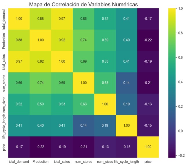
correlation plot
-
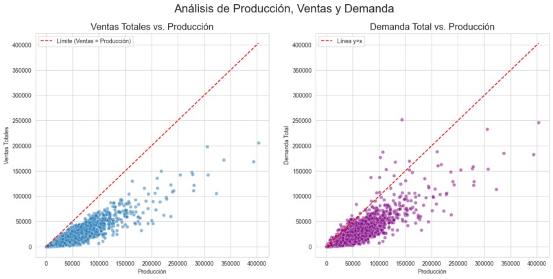
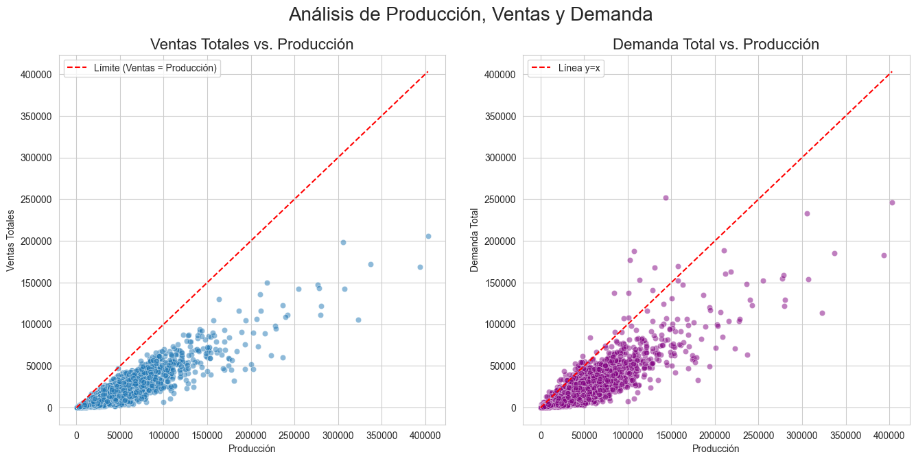
relation between sales, demand and production
-

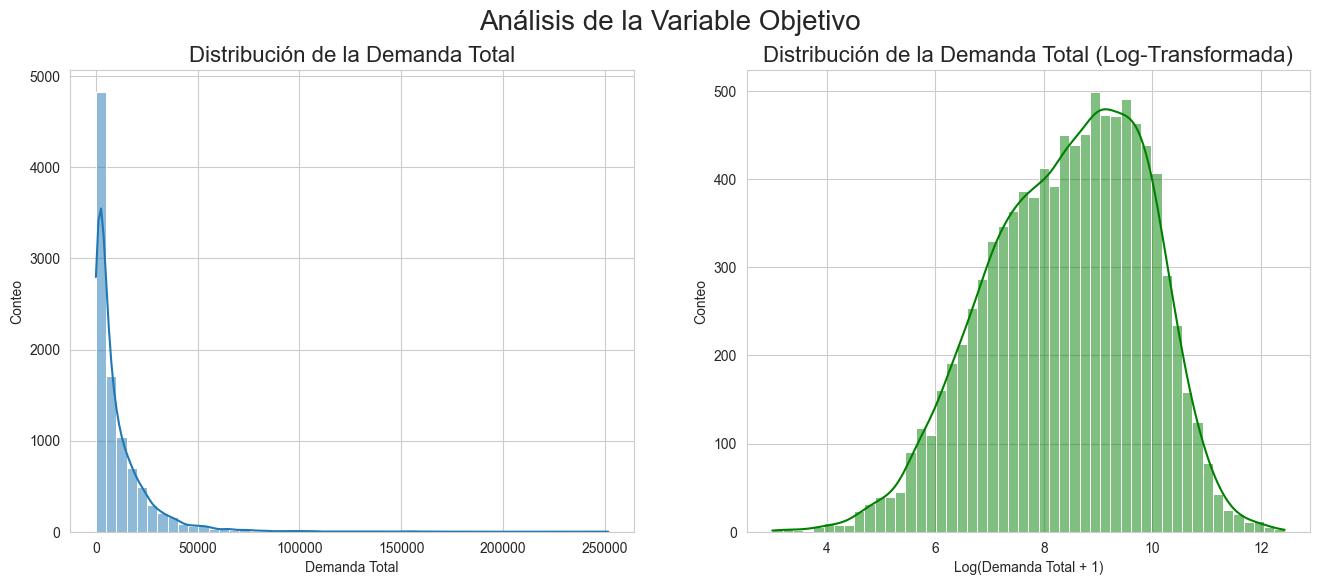
target variable anaylisis

Inspiration
Our main inspiration was the VAR business metric. The moment we realized that lost sales are dramatically more costly than excess inventory, the entire modeling strategy changed. Instead of predicting an average or a median, we designed a model that intentionally over-targets demand to avoid stockouts.
A second key source of inspiration came later: the correlation map. It clearly revealed that only a handful of numeric variables had real predictive power compared to the high-dimensional embeddings. This insight guided us to simplify rather than complicate, and ultimately made the model far more stable.
What it does
The system is a high-confidence production forecast model focused on maximizing VAR. Instead of trying to guess the “expected” demand, it predicts the 82nd percentile (P82) — a deliberately conservative estimate that minimizes the risk of under-production.
The model returns a single recommended production quantity for each product (ID). This value represents a strategic balance between demand uncertainty and business risk.
How we built it
Smart, Business-Driven Features:
We engineered features that contextualize each product within its competitive and historical environment:
- price_vs_trend (positioning the price relative to past demand patterns)
- category_scale (capturing category-level seasonality and size effects)
- last-season contextual demand (category and family)
This was crucial. These features ultimately contributed more to predictive power than any individual embedding component.
Embedding PCA Compression:
We reduced the combined text/image embeddings (≈200–300 dims) using PCA down to 64 components. This prevented embedding noise from overwhelming the simpler but more predictive numeric variables.
Log-Transform of the Target:
Weekly demand is extremely skewed. Applying a log-transform stabilized the variance, helped the quantile model isolate relative differences, and produced much more consistent forecasts.
Quantile LightGBM Model (α = 0.82):
The final production recommendation comes from a LightGBM Quantile Regressor, set to alpha=0.82. This allowed us to aim directly at the business objective: a high-confidence upper bound on demand.
Challenges we ran into
Embeddings vs. Numeric Features
The biggest challenge was balancing the 10 human-interpretable numeric features (e.g., price, num_stores, last-season demand) against the 200+ embedding features. Without PCA, embeddings completely dominated the model and degraded its behavior.
Finding the Right Quantile
Choosing the quantile wasn’t trivial. Too low → stockouts. Too high → overproduction. We used actual VAR behavior on a validation season to converge on P82.
The Correlation Map Realization
A crucial turning point came when we analyzed the correlation map:
price → moderate negative correlation num_stores, num_sizes → moderate positive correlation category_demand_last_season → extremely strong and consistent correlation
This showed two essential truths:
- We already had all the meaningful signal in the data.
- Most additional features tested were pure noise, explaining why model after model performed worse despite being “more complex”.
This insight led to simplification:
- Keep the core numeric features.
- Keep the reduced embeddings.
- Avoid adding extra engineered variables without clear statistical justification.
This was, arguably, one of the most important breakthroughs.
Accomplishments that we're proud of
We modeled the business metric, not the technical metric
Instead of optimizing MSE — which has almost nothing to do with VAR — we optimized directly for the quantile that maximizes business value.
The log-transform + PCA + quantile trio
This combination proved extremely stable:
- log-transform → smooths extreme demand volatility
- PCA → prevents embedding noise
- quantile regression → aligns directly with VAR
A simple, robust, justifiable model
In a context with limited signal and high noise, simplicity won. We arrived at a model that is: fast, interpretable, reproducible and strategically aligned.
What we learned
Always model the real business objective
Technical metrics are only proxies. In this case, MSE was misleading — VAR is what matters.
Log-transforming demand is non-negotiable
Raw demand is too skewed. Log-transformation is essential to stabilize both training and predictions.
High-quality features beat raw embeddings
The correlation map showed this repeatedly. A few smart features can outperform hundreds of embedding components.
Complexity can be counterproductive
Almost every “fancier” experiment made the model worse:
more features, more interactions, more embedding dimensions, more complex pipelines. Noise, not signal.
What's next for EliBoost v.2 FT for MANGO
Fine-tune the Quantile: Is 0.82 really the perfect number? We'd test 0.81, 0.83, etc.
Hyperparameter Tuning: Use a tool like Optuna to find the best LightGBM settings.
GroupKFold Validation: Re-train the model using cross-validation grouped by id_season to make it even more robust for future seasons.


Log in or sign up for Devpost to join the conversation.