Eisengrau
GB imbalance prices swing hard. Eisengrau lines up their drivers using only data known at the time, backtests 14 transparent models and shows which forecasts deserve trust, at which lead time.
Inspiration
Every half hour, any GB generator, supplier or battery that misses its contracted position settles the difference at the imbalance price. That price is volatile. On our data its forecast errors are heavy-tailed, and big moves cluster together.
The data that explains it is public, but it's spread across Elexon, NESO and weather services. Each source has its own cadence and units, and forecasts are re-published dozens of times before delivery. That makes backtests easy to get wrong: use a forecast published after the period it predicts and a model looks far better than it ever could have been. Most dashboards also make claims like "model X is best" or "80% confidence" without testing them.
We wanted a tool that answers a narrower but more useful question: which forecasts can I actually trust, and how far ahead?
What it does
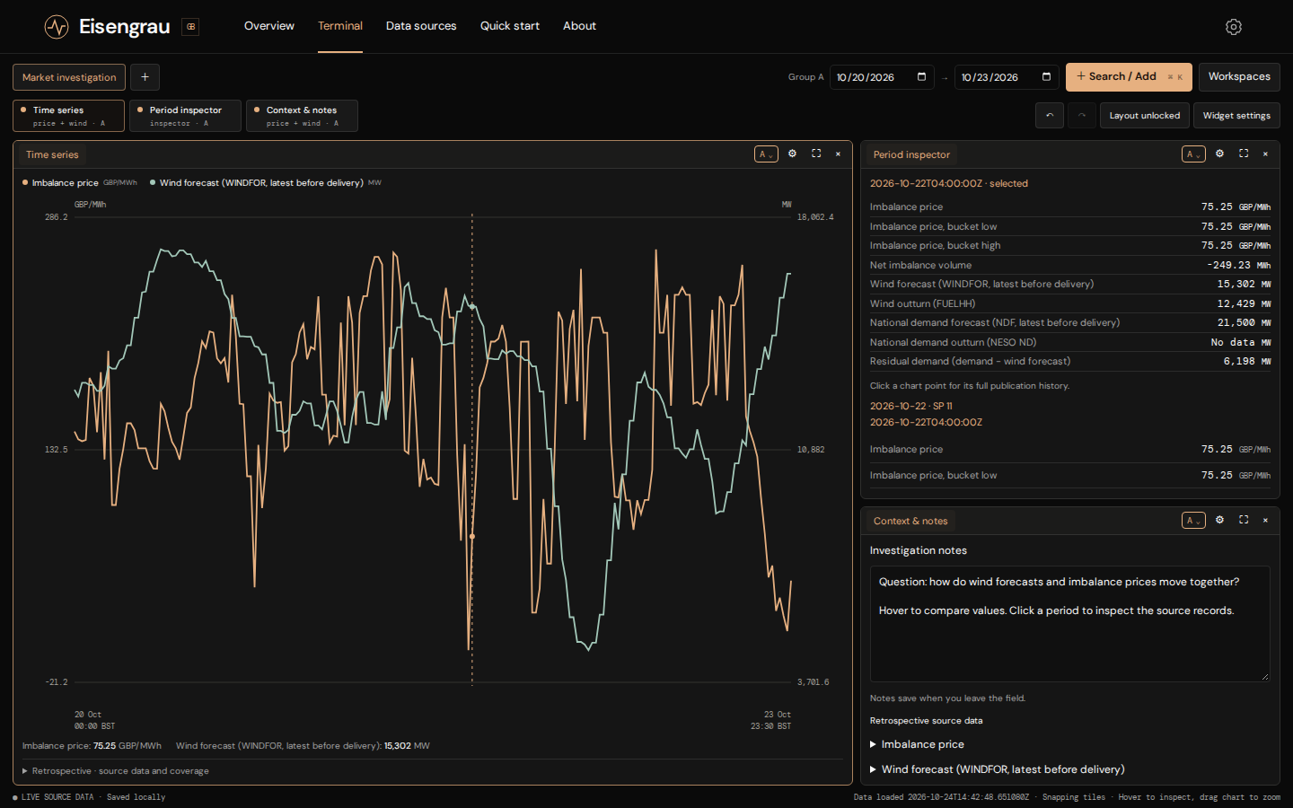
One time-aligned view of the market. Eisengrau puts imbalance prices, net imbalance volume, wind and demand forecasts, wind and demand outturns, residual demand and regional weather on a single settlement-period grid. The data runs from January 2024 to October 2026. Clock-change days with 46 or 50 periods are handled correctly.
Honest history. Every forecast is the last version published before delivery, so the past shows what the market actually knew. Every version is still kept for inspection. Data that is only retrospective, such as archived weather without publication times, is labelled as such.
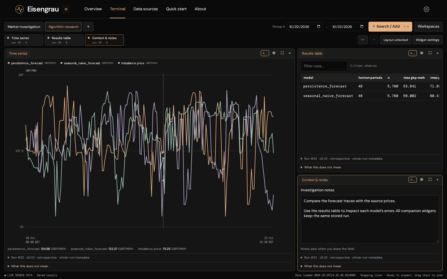
Forecasts tested properly. Rolling-origin backtests compare 14 transparent statistical models. Each day the models are refitted on the previous 28 days and forecast the next 48 periods. Each model is scored on:
- error at every lead time: MAE, RMSE, wMAPE, sMAPE, MASE and RMSSE
- whether its 80% and 95% bands actually contain 80% and 95% of outcomes
- interval score, MSIS and pinball loss, with results for every fold
Explanation, not just numbers. Correlograms show how price moves with residual demand and wind, and residual diagnostics test each model's assumptions.
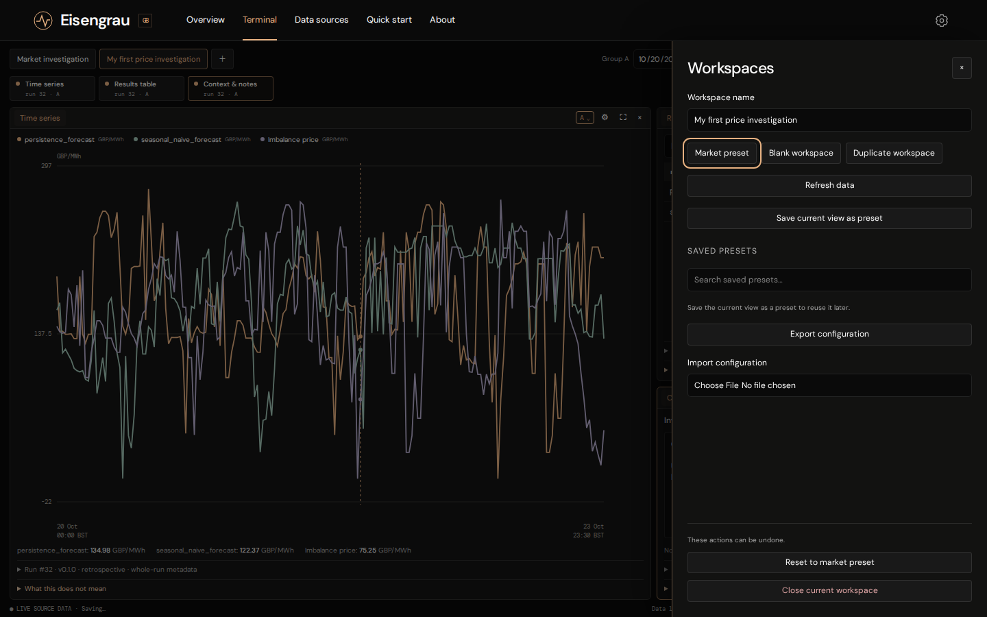
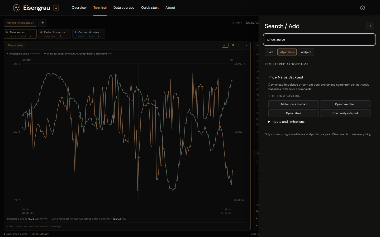
An AI analyst in the Terminal. The Terminal is a dockable workspace of linked charts, tables and comparisons. Its AI agent investigates questions with the same data and tools as the dashboard and cites the runs it used. It rebuilds the workspace around what it found; every change is validated and can be undone. Expensive computations need your explicit approval.
Pages
- Overview: price, wind, demand and weather for any day on one screen, with separate price and GW axes and instant hover readouts
- Terminal: the analysis workspace and AI agent
- Sources and Status: every dataset's provider, coverage, load time and freshness
- About: an animated explanation of the GB market and the project
The algorithms
Every analysis is a classical statistical method. None is a trained black box: parameters are estimated from the data on each run, and every result is stored with the exact data it used.
| Analysis | Methods |
|---|---|
| Baseline backtest | Naive (last value), seasonal naive (same period yesterday and last week), Naive2 (seasonally adjusted naive), drift, mean of the window, 48-period moving average, weighted moving average |
| Statistical forecast backtest | ETS(A,N,A): exponential smoothing with additive error, no trend and an additive daily season. ARIMA(2,0,1) on daily-differenced prices. Both measured against a daily seasonal naive |
| Regression backtest | Linear trend, half-hourly seasonal dummies, daily Fourier-term regression, and a calendar regression with daily and weekly harmonics on GB clock time |
| Day-ahead forecast | AutoETS and AutoARIMA with automatic model selection on the last 28 days, forecasting every period of the next settlement day (46, 48 or 50), against a seasonal naive |
| Driver correlograms | Autocorrelation and partial autocorrelation of price; cross-correlation of price with residual demand and the wind forecast at each lag |
| Residual diagnostics | Ljung–Box, Durbin–Watson, Jarque–Bera and ARCH-LM tests on the ETS and ARIMA residuals |
| Rolling signals | Trailing 24-hour simple, linearly weighted and exponential means; 24-hour variance, standard deviation, median and RMS; 7-day 10th and 90th percentiles; period and daily changes. Each value uses only past prices |
| Wind–price correlation | Trailing 7-day Pearson correlation between the wind forecast and the price |
| Persistence backtest | Persistence and same-period-last-week forecasts, with a table of the worst misses |
| Calendar Fourier terms | Sine and cosine terms of Europe/London clock time, the seasonal basis of the calendar regression |
What we found
These are the stored results for the eight weeks to 23 October 2026. MAE is in £/MWh.
| Model | MAE, 30 min ahead | MAE, 24 h ahead | 80% band coverage |
|---|---|---|---|
| Naive (repeat last price) | 18.5 | 54.2 | 0.99 |
| ETS(A,N,A) | 22.5 | 51.7 | 0.94 |
| ARIMA(2,0,1), daily difference | 34.8 | 54.8 | 0.80 |
| Fourier regression | 44.9 | 40.8 | 0.99 |
| Mean of last 28 days | 43.7 | 39.0 | 0.77 |
| Seasonal naive (yesterday) | 59.4 | 54.2 | 0.78 |
- The best model depends on the lead time. Half an hour ahead, repeating the last price wins. A day ahead, a plain 28-day average beats everything else. ETS has the best average over the whole day (MASE 0.85) only because it is strong in the first few hours.
- Yesterday is a poor guide to today. Copying yesterday's price shape is worse than simply repeating the last price.
- Most confidence bands tell you nothing. Nine of the 14 models have "80%" bands that contain 99% of prices.
- Errors break the usual assumptions. The residual tests show heavy tails and volatility clustering (ARCH effects), so Gaussian bands are too narrow in volatile spells and too wide in calm ones.
- The drivers matter. Price correlates at +0.62 with residual demand (demand minus wind) and −0.46 with wind, both far outside the ±0.04 noise band. Correlation is not causation, and we don't claim it is.
How we built it
- Data: Elexon BMRS (imbalance prices, WINDFOR wind forecasts, NDF demand forecasts, FUELHH outturn), NESO historic demand, and Open-Meteo archived forecasts for six wind regions from Dogger Bank to the Moray Firth.
- Database: Tiger Data (TimescaleDB). Raw tables feed views with one row per settlement period. Continuous aggregates pick the latest pre-delivery forecast; before them, forecast series were 5–25× slower.
- Analysis: pure-Python statistical models behind a common contract that declares each algorithm's inputs, outputs, units and tables. Results are stored with the datasets and load times they used, so a stale result is detectable. A scheduled job reruns stale analyses every three hours.
- Backend: Python, FastAPI, pandas and NumPy.
- Frontend: SvelteKit, TypeScript, Tailwind, D3 charts and a Three.js globe on the About page.
- AI agent: GPT-5.4 mini via OpenRouter, using typed tools over the existing API. Proposed layouts are compiled and validated before they're applied; on failure the agent gets two repair attempts.
- Ops: Docker, with GitHub Actions deploying to a Vultr VPS (development and production sites).
- Testing: pytest, Vitest and Playwright.
Challenges we ran into
- "Latest forecast" is harder than it sounds. Each WINDFOR publication re-issues the previous ~27 hours, and some demand periods have about 60 forecast versions. WINDFOR is also hourly while settlement is half-hourly. Picking the right value for each period without leaking future information, and doing it fast, took continuous aggregates and careful view design.
- Model fitting is slow. A full ETS and ARIMA backtest took 109 seconds. Running the independent fits in parallel cut it to 31 seconds on four workers. We also cache each fold, so a daily refresh refits only the new day instead of all 56.
- Gaps and clock changes. One missing price should cost one fold, not a whole backtest. Daylight-saving days have 46 or 50 periods, and on them seasonal lags point an hour off; those fits carry a warning. One of those days, 25 October, fell during the hackathon.
- Letting an AI change the screen safely. Layout changes had to be all-or-nothing and undoable. The agent also had to cope with races against manual edits and must never claim to have added a table that failed to render.
Accomplishments that we're proud of
- Every number on this page comes from stored, reproducible runs, and each run records exactly which data it used.
- The point-in-time discipline: the history shows what the market actually knew, not what we know now.
- Results that go against the usual story, such as useless confidence bands and a simple average winning a day ahead, reported plainly instead of hidden.
- An AI agent that shows its evidence and can't run expensive computations without your approval.
What we learned
- On short horizons, simple models are very hard to beat. Any forecast should state its lead time.
- Prediction intervals must be checked against outcomes. Wide bands look safe but carry no information.
- More structure doesn't automatically help. ARIMA on daily-differenced prices barely beat the seasonal naive it is built on, and ETS's fitted daily season never updated.
- Data lineage (what was known, when, and from which load) matters as much as the model.
What's next for Eisengrau
- Use the drivers in the forecasts. The models currently use price history only; wind, demand and weather appear on charts but don't feed any forecast yet.
- Use the data already loaded. That includes transmission demand forecasts, NESO embedded wind and solar forecasts, and ERA5 reanalysis.
- Better uncertainty. Volatility-aware and calibrated intervals, and longer evaluation windows across seasons.
- State-space models such as local-level and structural models with Kalman filtering.
- A Methods page explaining each algorithm, and a synoptic weather map with wind, pressure, fronts and isobars.
- Scenario and stress testing for decisions such as battery dispatch or hedging.
Eisengrau is an analysis and decision-support tool, not trading advice. The results above come from one autumn period in one market.
Built with
Python · FastAPI · pandas · NumPy · psycopg · Tiger Data · TimescaleDB · PostgreSQL · SvelteKit · Svelte · TypeScript · Tailwind CSS · D3.js · Three.js · OpenRouter · GPT-5.4 mini · Docker · GitHub Actions · Vultr · pytest · Vitest · Playwright · Elexon BMRS · NESO Data Portal · Open-Meteo
Built With
- actions
- bmrs
- css
- data
- docker
- elexon
- fastapi
- github
- gpt-5.4
- neso
- numpy
- openrouter
- pandas
- playwright
- portal
- postgresql
- psycopg
- pytest
- python
- svelte
- tailwind
- tiger
- timescaledb
- typescript
- vultr

Log in or sign up for Devpost to join the conversation.