-
-

Logo
-
-
-
-
-
-
-
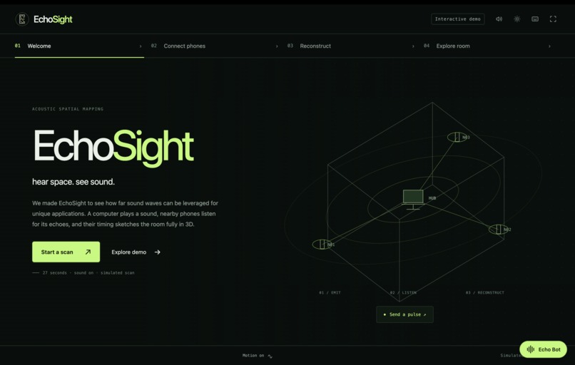
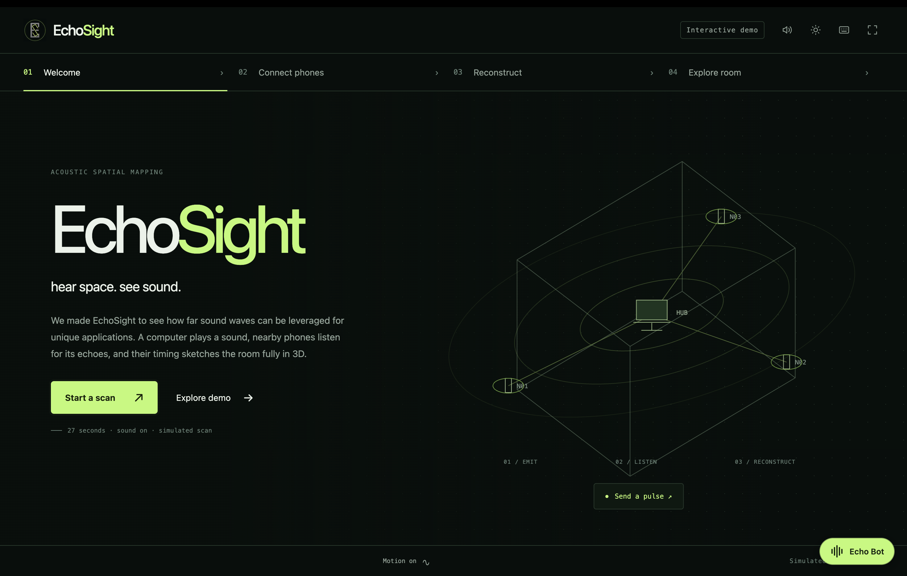
Initial UI
-
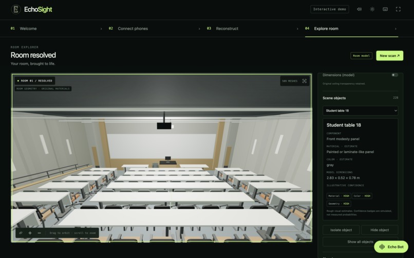
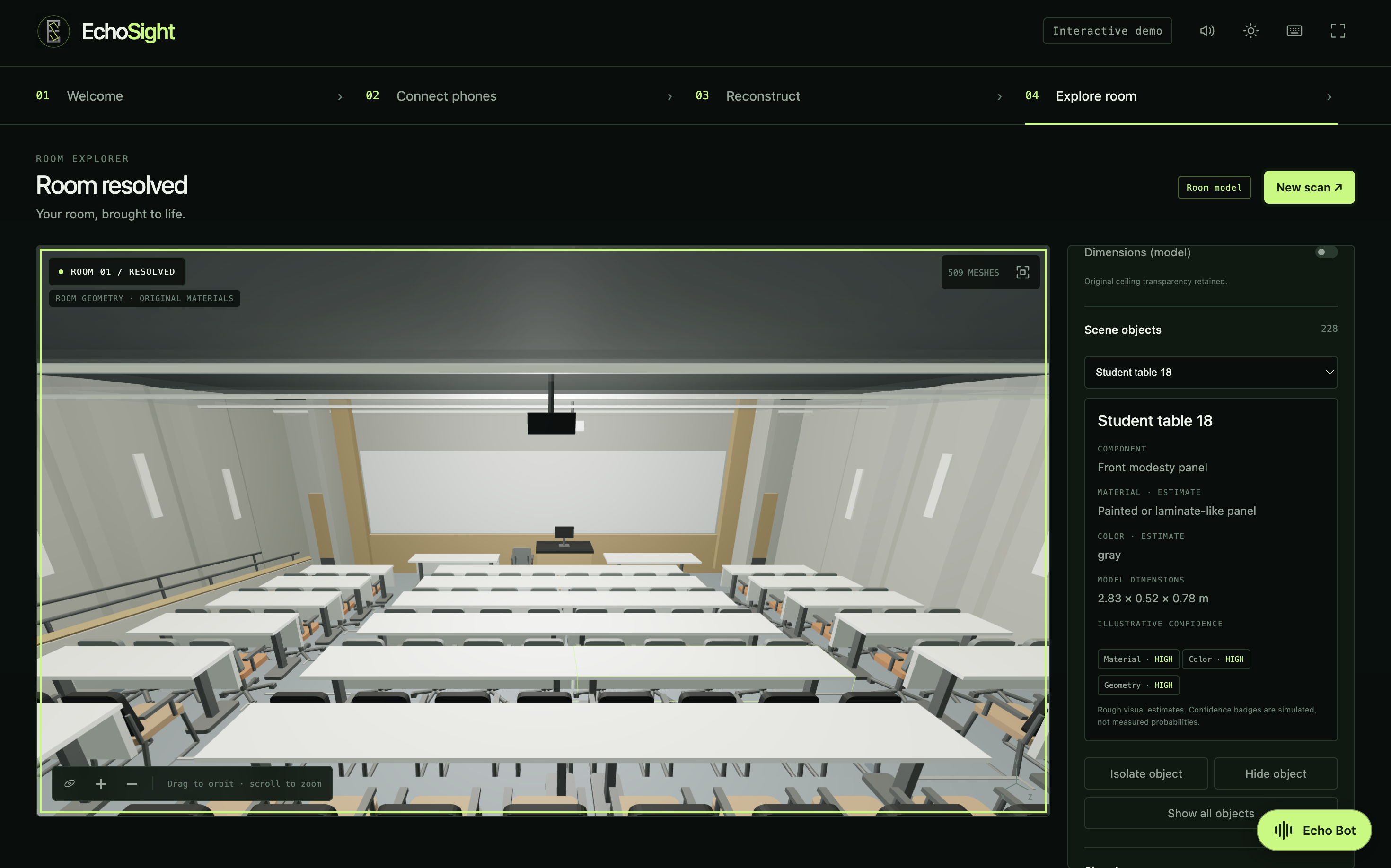
3D model of NCB 160 with an overall accuracy score of 97.1%
-
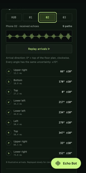
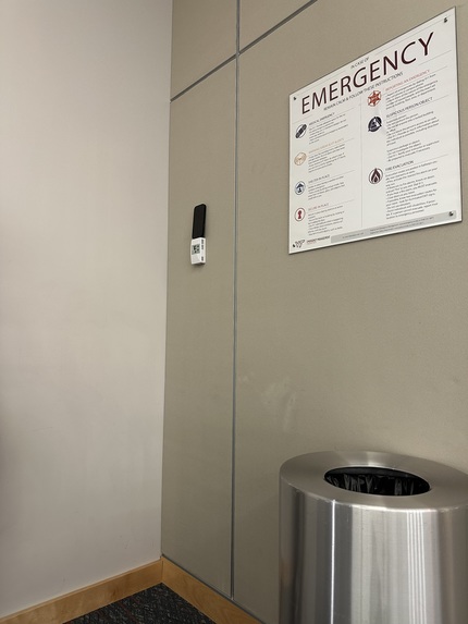
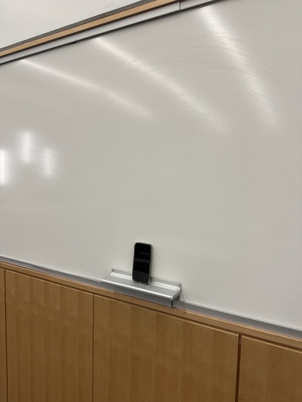
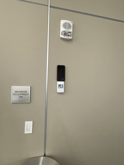
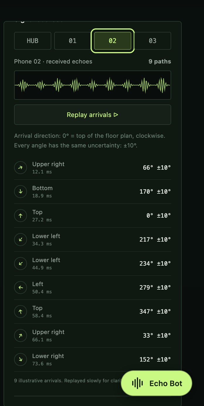
3D sensor analysis of the sound waves (incl reflections) using iPhones

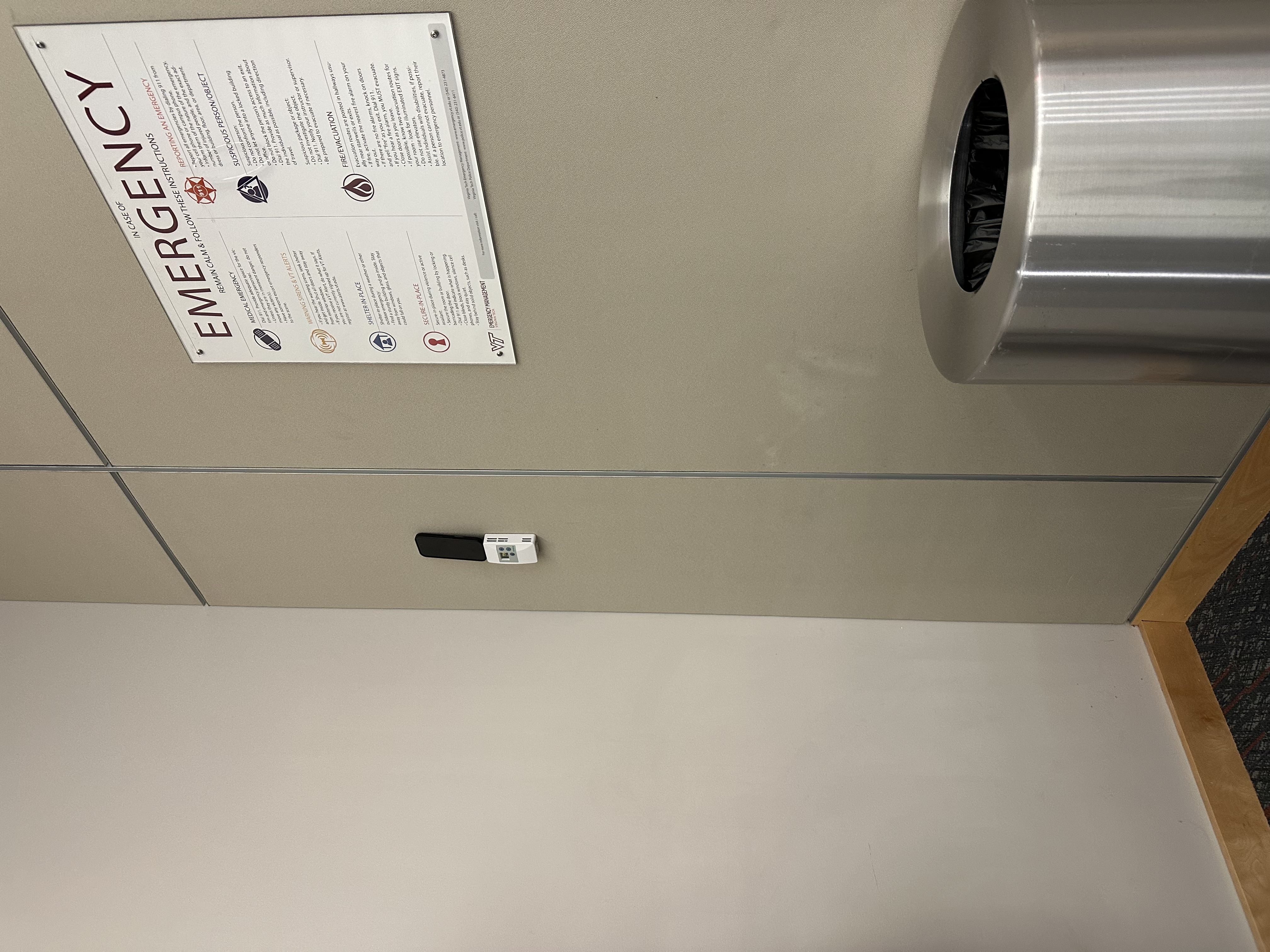
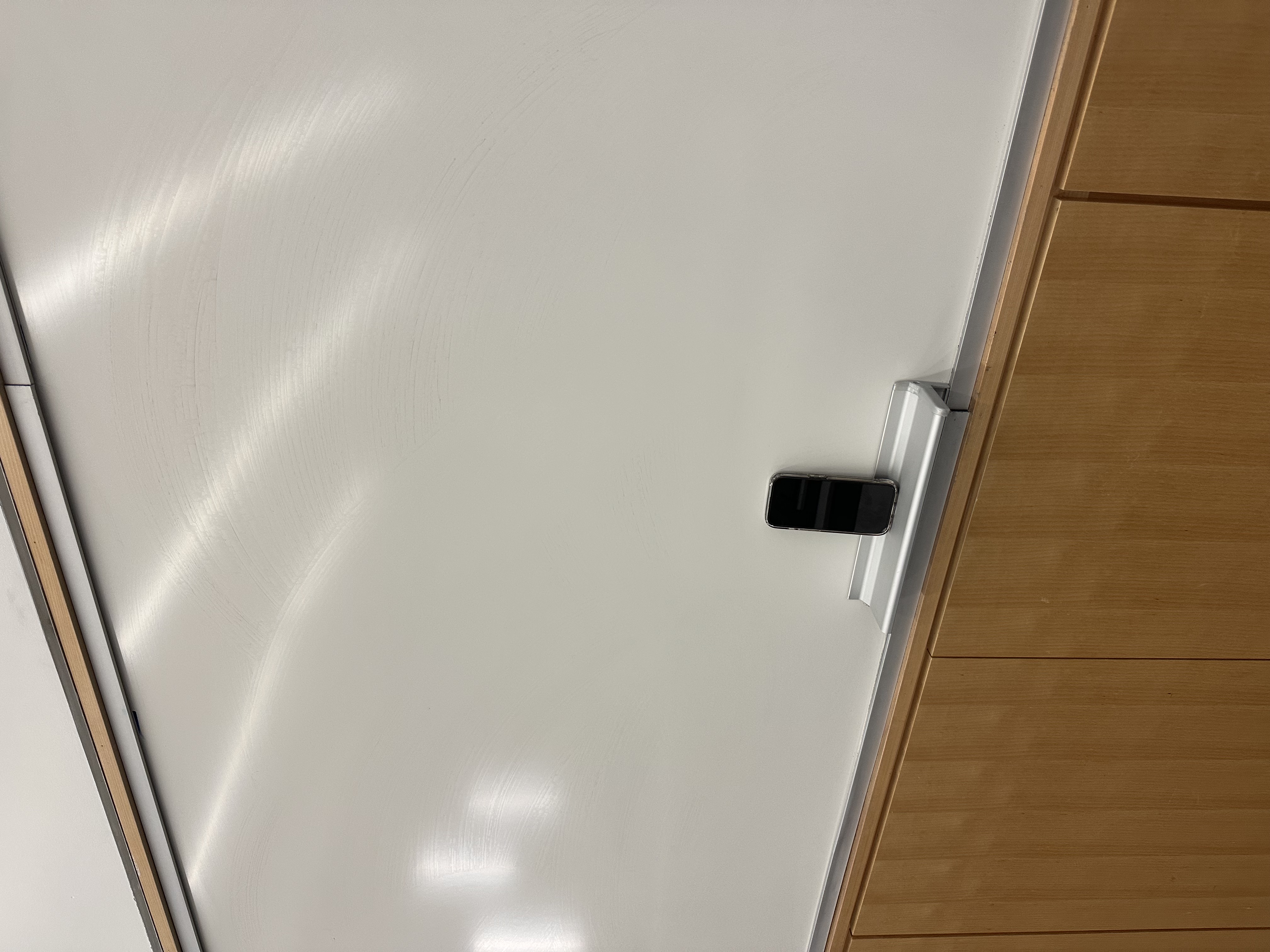
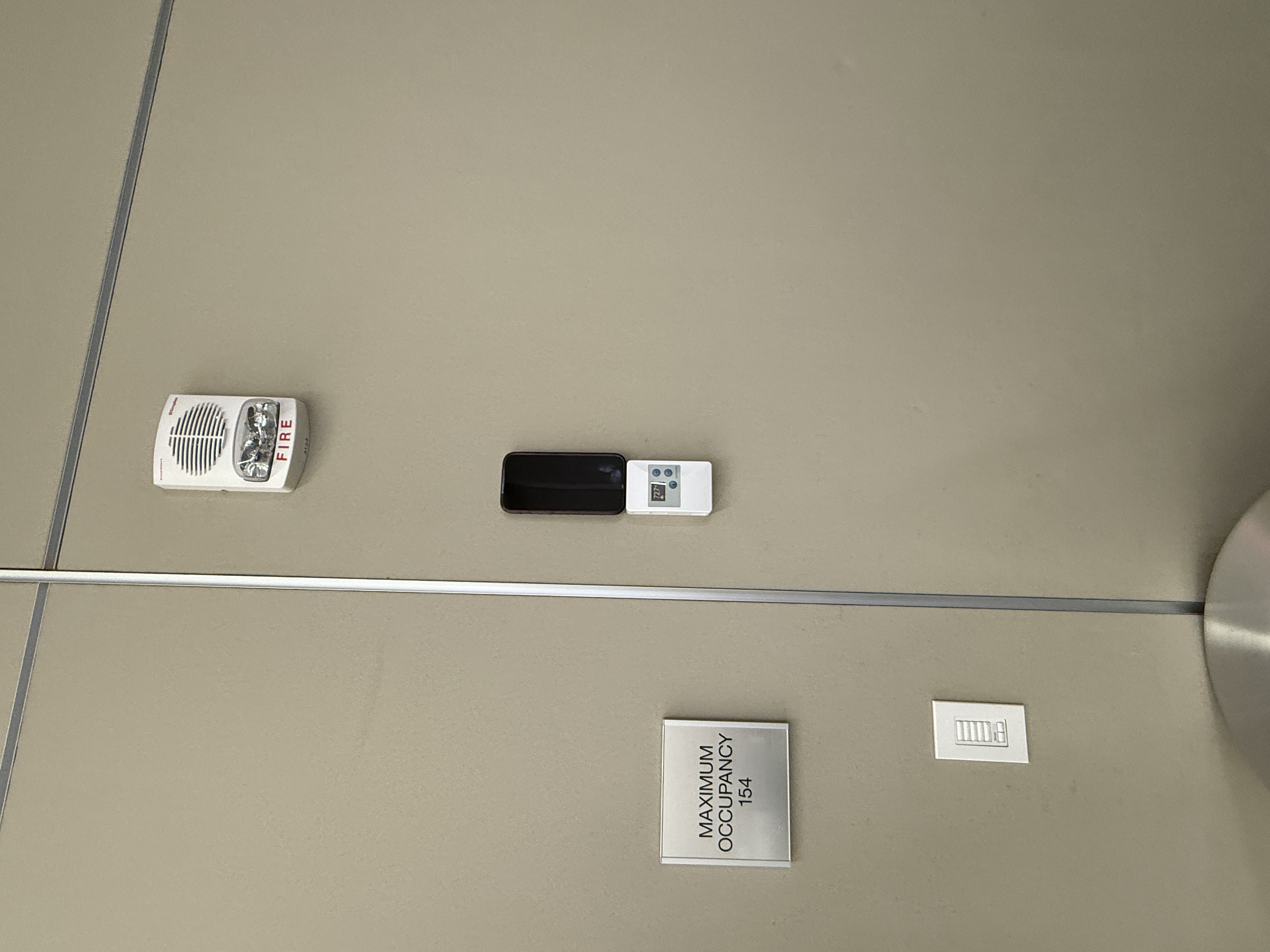

EchoSight
Inspiration
EchoSight started with a simple question:
Can we reconstruct a 3D environment using only sound and devices people already own?
Traditional spatial mapping often relies on cameras, sonar, or dedicated depth sensors. We wanted to explore a different sensing modality entirely: acoustics.
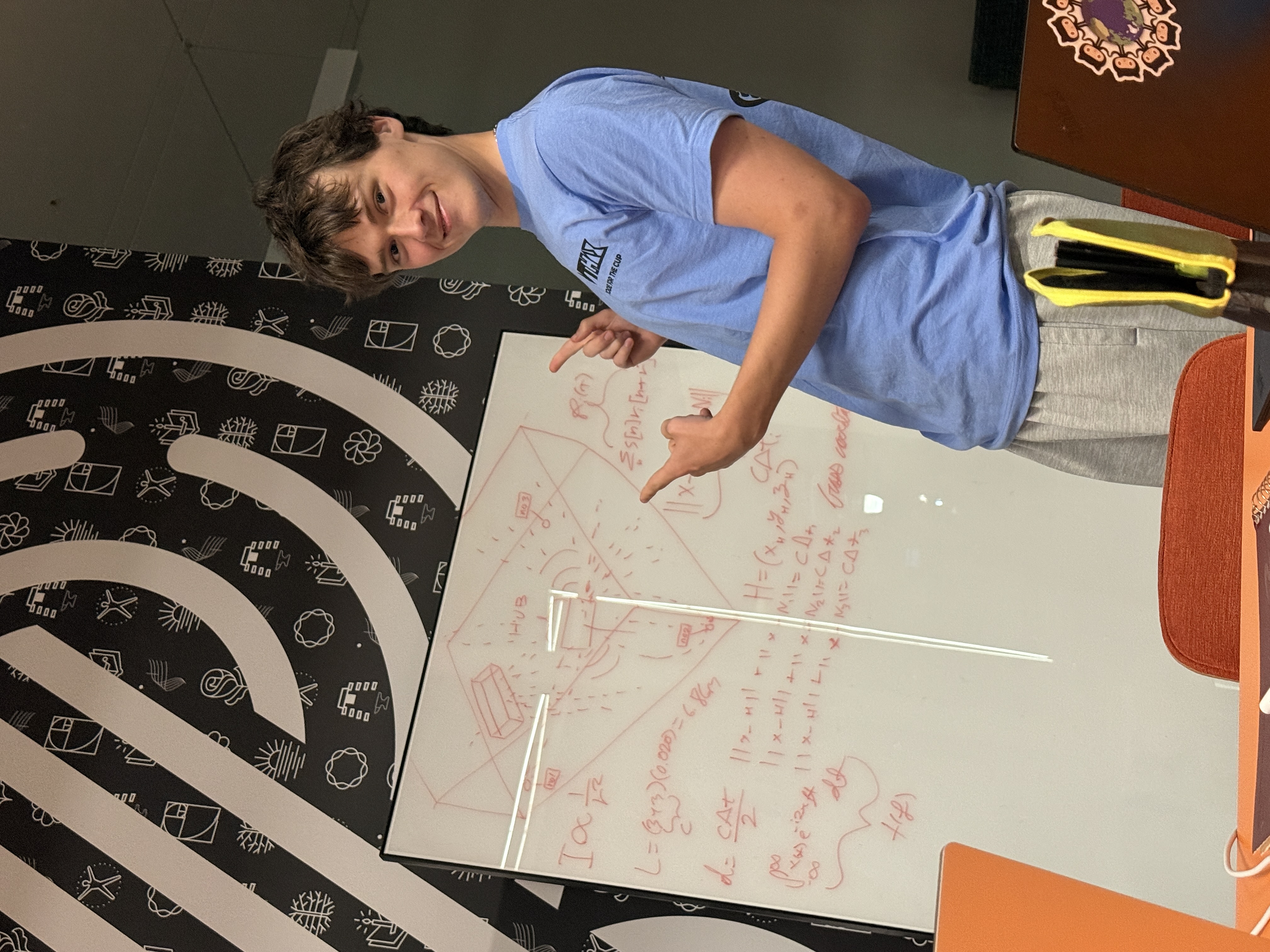
A laptop emits a known sound. Several iPhones record both the direct signal and the echoes returning from the environment. Those reflections encode information about the geometry that produced them.
EchoSight asks an inverse-physics question:
Given the sound we measured, what physical environment could have produced it?
What it does
EchoSight turns acoustic reflections into estimates of the dominant planar surfaces of a room.
For microphone $$m$$, the recorded signal is modeled as
$$ y_m(t) = (x \ast h_m)(t) + n_m(t), $$
where $$x(t)$$ is the known acoustic probe, $$h_m(t)$$ is the room impulse response, and $$n_m(t)$$ represents noise and unmodeled effects.
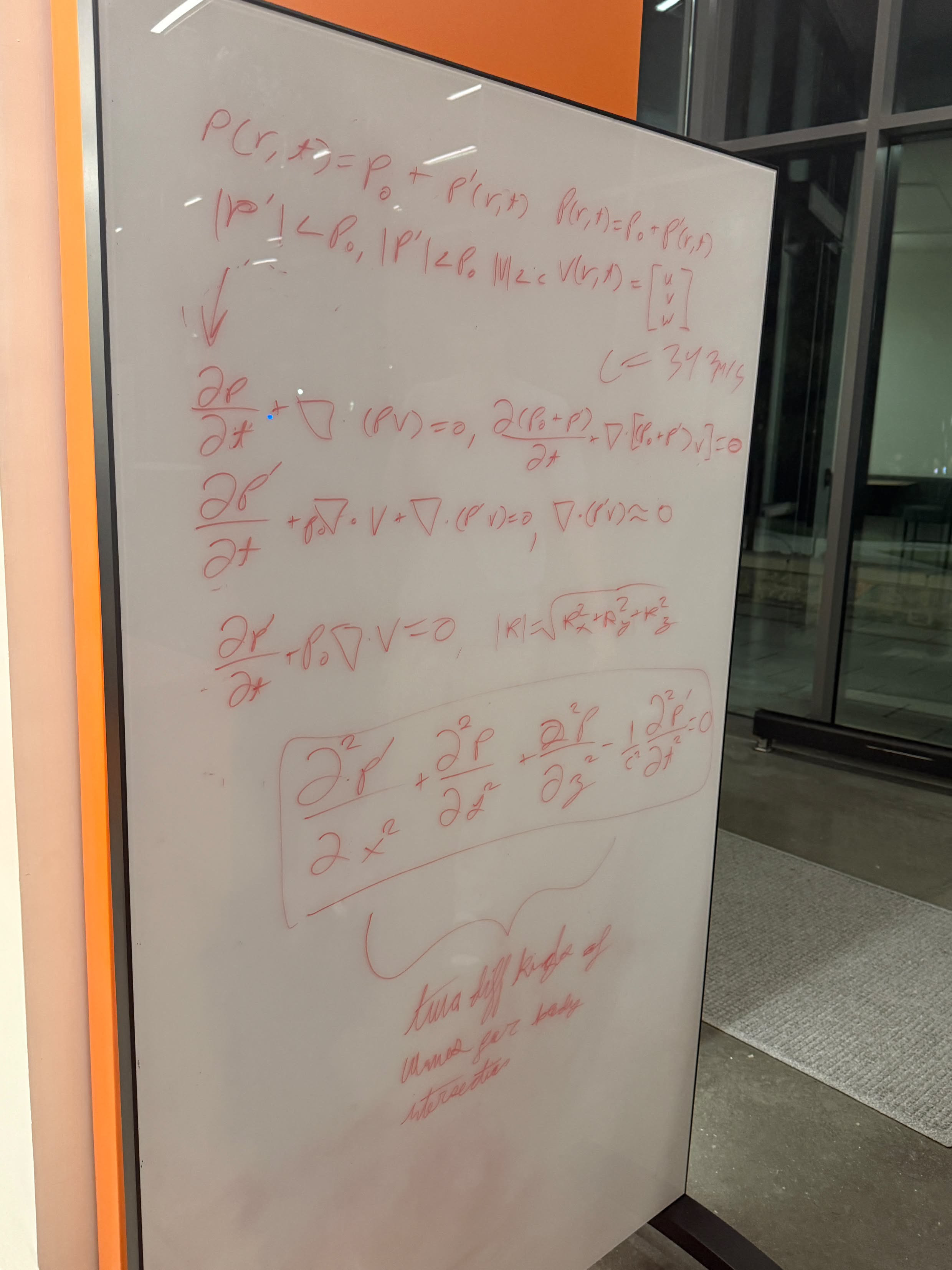
We transmit repeated 2–15 kHz chirps at 48 kHz, then correlate each recording with the known probe. This produces sharp peaks corresponding to the direct arrival and strong reflected arrivals.
The processing pipeline is:
Acoustic Probe → Recording → Clock Calibration → Correlation → Echo Detection → Geometry Solver → 3D Reconstruction
The key insight is that an echo delay is not simply a wall distance.
For a reflection from plane $$k$$ recorded at receiver $$m$$,
$$ \Delta\tau_{mk} = \frac{ \lVert r_m - q_k \rVert - \lVert r_m - s \rVert }{c}, $$
where $$s$$ is the source position, $$r_m$$ is the receiver position, $$q_k$$ is the corresponding image source, and $$c$$ is the speed of sound.
Equivalently,
$$ \lVert r_m - q_k \rVert = \lVert r_m - s \rVert + c \Delta\tau_{mk}. $$
Each receiver therefore constrains where the image source can exist. Combining consistent measurements from multiple viewpoints lets us estimate that image source and recover the reflecting surface.
In our current evaluation, source and receiver positions are supplied to the geometry solver as known inputs. Joint acoustic estimation of device positions is a future extension.
How we built it
1. Acoustic probing
The laptop repeatedly emits a broadband chirp spanning approximately 2–15 kHz.
Because the emitted waveform is known, each phone recording can be correlated with the original probe to estimate when the direct signal and later reflections arrived.
Broadband probing gives substantially more timing information than trying to infer geometry from arbitrary environmental sound.
2. Clock-rate calibration
Different phones do not share a perfectly identical audio clock.
We model receiver-local time relative to the source timebase as
$$ u_m(t) = a_m t + b_m, $$
where $$a_m$$ captures relative clock rate and $$b_m$$ captures timing offset.
Repeated direct arrivals allow us to estimate the clock-rate factor $$a_m$$.
For an echo-to-direct interval measured on the same receiver,
$$ \Delta u_m = u_m(t_{\text{echo}}) - u_m(t_{\text{direct}}) = a_m (t_{\text{echo}} - t_{\text{direct}}), $$
the constant offset $$b_m$$ cancels.
The corrected physical delay is therefore
$$ \Delta\tau_m = \frac{\Delta u_m}{\hat a_m}. $$
This distinction mattered: the phones do not need perfectly synchronized recording start times for a within-device echo delay, but sampling-rate mismatch and clock drift still distort inferred path lengths if they are ignored.
3. Echo detection
After correlation, EchoSight identifies the direct arrival and candidate reflection peaks.
Not every peak is useful. Noise, clipping, overlapping reflections, multipath, and device response can all produce misleading measurements.
Measurements therefore have to survive signal-quality and geometric consistency checks before being treated as evidence for a surface.
4. Image-source geometry
A plane is represented as
$$ \mathcal{P}_k = \left\lbrace x \in \mathbb{R}^3 : n_k^{\mathsf T} x = b_k \right\rbrace, \qquad \lVert n_k \rVert = 1. $$
Reflecting the real source $$s$$ across that plane produces an image source
$$ q_k = s + 2\left(b_k - n_k^{\mathsf T} s\right) n_k. $$
Instead of reasoning about every reflected ray independently, we solve for the virtual source that could have produced a consistent set of measured path lengths.
Once $$q_k$$ is estimated, the physical reflector is the plane halfway between the real source and its image, perpendicular to the vector connecting them.
The normal direction is proportional to
$$ n_k \propto q_k - s, \qquad\text{i.e.}\qquad n_k = \frac{q_k - s}{\lVert q_k - s \rVert}, $$
and the plane passes through the midpoint
$$ p_k = \frac{s + q_k}{2}, \qquad\text{so}\qquad b_k = n_k^{\mathsf T} p_k. $$
This converts acoustic timing measurements into an actual geometric surface.
Acoustic material evidence
Geometry is EchoSight's core reconstruction problem. We are also exploring how the frequency-dependent behavior of each accepted echo can provide evidence about the type of surface that reflected it.
For an echo associated with a reconstructed plane, we compare its spectrum with the direct-path spectrum while compensating for first-order path-length spreading:
$$ F_{mk}(f) = \frac{ \hat H_{mk}^{\mathrm{win}}(f) }{ \hat H_{m0}^{\mathrm{win}}(f) } \frac{L_{mk}}{L_{m0}}. $$
In practice, low-energy frequency bins must be rejected or regularized because dividing by a weak reference spectrum is unstable.
The physical quantity motivating this feature is the pressure reflection coefficient. For an ideal locally reacting surface with impedance $$Z_b(f)$$ and incidence angle $$\theta$$,
$$ R(f,\theta) = \frac{ Z_b(f)\cos\theta - \rho_0 c }{ Z_b(f)\cos\theta + \rho_0 c }. $$
Its magnitude and phase depend on frequency and surface properties.
But a weak measured echo does not automatically mean that a surface is highly absorptive.
Measured amplitude is also affected by source and microphone directivity, scattering, transmission, incidence angle, automatic gain behavior, finite-window effects, device frequency response, and calibration error.
For that reason, EchoSight treats the measured spectrum as an effective acoustic feature, not as an absolute absorption coefficient.
Appearance estimation
Sound does not directly measure pigment or surface color.
Instead, appearance can only be inferred probabilistically by combining acoustic material evidence with geometry and contextual information.
Let $$Y$$ represent acoustic evidence, $$G$$ geometry, $$C$$ contextual information, $$M$$ material class, and $$A$$ appearance. A possible model is
$$ P(A \mid Y, G, C) = \sum_{M} P(A \mid M, C) P(M \mid Y, G, C). $$
The goal is therefore not to claim that an acoustic measurement uniquely reveals a paint color.
Instead, the system can preserve several plausible color-family or appearance hypotheses when the evidence is ambiguous.
For example, if two visually different finishes are acoustically indistinguishable under the available measurements, EchoSight should preserve both possibilities rather than invent certainty.
Any visualization that maps an acoustic statistic directly to hue is explicitly labeled acoustic false color. It represents the measurement itself, not the real-world pigment of the surface.
A major next step is testing whether acoustic material features actually improve appearance prediction over a context-only baseline on held-out rooms, devices, and surface specimens.
Challenges we ran into
Different device clocks
One of the biggest technical challenges was using recordings from independent phones.
Even when two devices nominally record at 48 kHz, their physical audio clocks are not perfectly identical. Small rate errors accumulate over time and can become meaningful spatial errors when time delay is converted into acoustic path length.
This led us to explicitly model and correct relative clock rate instead of assuming every device shared an identical timebase.
Echo association
Detecting an echo is easier than determining which physical surface generated it.
A peak detected on one phone and a peak detected on another phone are not automatically reflections from the same wall.
The reconstruction therefore has to look for groups of measurements that are simultaneously compatible with a common image source and reject combinations that violate the geometry.
Real acoustics are messy
Real rooms contain overlapping reflections, diffuse scattering, furniture, device directivity, background noise, clipping, reverberation, and surfaces that do not behave like ideal infinite planes.
That gap between a clean physical model and a real room became one of the most important parts of the project.
Accomplishments that we're proud of
We built a complete physics-driven path from a known acoustic waveform to candidate 3D reflector planes:
Probe → Correlation → Timing → Clock Correction → Echo Constraints → Image Sources → Planes
In a model-consistent twelve-view synthetic validation, our solver produced six predicted planes that matched all six reference planes under our evaluation threshold.
Plane-normal errors ranged from
$$ 0.049^\circ \quad\text{to}\quad 0.486^\circ, $$
and plane-offset errors ranged from
$$ 0.12\text{ mm} \quad\text{to}\quad 18.39\text{ mm}. $$
These numbers characterize the geometry solver under our synthetic evaluation conditions. They are not claims of real-room centimeter or millimeter accuracy.
We also tested important failure cases.
Clipped inputs were rejected, while degenerate coplanar and null controls returned no definitive plane rather than confidently producing a false reconstruction.
For an inverse problem, knowing when the evidence is insufficient is just as important as producing an answer when it is sufficient.
What we learned
The biggest lesson was that time resolution, acoustic resolution, and reconstruction accuracy are different things.
At 48 kHz, one sample corresponds to approximately
$$ \frac{c}{f_s} \approx \frac{343\text{ m/s}}{48000\text{ Hz}} \approx 7.1\text{ mm} $$
of acoustic path length.
But the 13 kHz probe bandwidth gives a characteristic correlation scale on the order of
$$ \frac{c}{B} \approx \frac{343\text{ m/s}}{13000\text{ Hz}} \approx 2.6\text{ cm}. $$
Neither number is the final positional accuracy of EchoSight.
Sub-sample delay estimation can provide timing estimates finer than one sample, while noise, bandwidth, echo overlap, receiver geometry, clock error, sound-speed uncertainty, incorrect echo association, and model mismatch can all reduce final reconstruction accuracy.
We also learned that the speed of sound itself is part of the measurement model. A value near 343 m/s is reasonable around room temperature, but real-world reconstruction should account for environmental conditions rather than treating $$c$$ as perfectly fixed.
Most importantly, we learned that an echo is not a distance measurement by itself.
The quantity
$$ c \Delta\tau_{mk} = \lVert r_m - q_k \rVert - \lVert r_m - s \rVert $$
is an excess acoustic path length.
Recovering the physical surface that produced it requires multiple measurements, correct timing, and a geometric model that explains those measurements simultaneously.
What's next for EchoSight
The next step is taking the system from controlled and synthetic validation into increasingly difficult measured environments.
We want to:
- validate reconstructed geometry against rooms with independently measured ground truth,
- improve clock-rate estimation across different phone models,
- account for temperature-dependent sound speed,
- characterize speaker and microphone frequency responses,
- improve robustness when multiple echoes overlap,
- investigate joint estimation of unknown device positions,
- evaluate material classification using calibrated multi-view acoustic measurements,
- test whether acoustic material information provides measurable improvement over context alone for appearance inference,
- and quantify uncertainty so EchoSight can distinguish between what it knows, what it suspects, and what the acoustics cannot determine.
Long term, the goal is bigger than detecting individual echoes.
We want EchoSight to continuously solve the inverse problem:
Given the sound we measure, what physical environment could have produced it?

Log in or sign up for Devpost to join the conversation.