Oh, Well.

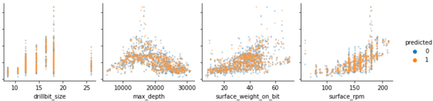
Performance of Random Forest Model predicting Rate of Penetration (2)
Parallel Coordinate Plot of Local Importance
Collinearity Analysis (1)
Collinearity Analysis (2)
Parallel Coordinate Plot of Potential Regressors
Performance of Random Forest Model predicting Rate of Penetration (1)

Inspiration

Offshore drilling can be a time-, labor-, and resource- intensive endeavor. Investment into new underwater rigs poses unique challenges to financiers, as tens of thousands of feet and rock must be displaced before acquisition of the precious oil. Luckily, insight gleaned from careful analysis of empirical data can minimize cost, ultimately maximizing profit and ensuring a competitive market position for the data fluent. Here, we attempt to model the role of controllable and preexisting drilling parameters in determining the rate of penetration in drill sites. With this model, we hope to assist in the creation of of the ultimate ‘Drilling Roadmap’.

What it does

Our model predicts the rate of penetration as a function of drilling parameters, controllable and known, of offshore wells.

How we built it

Our Workflow

Step 0: Cleaning and Understanding Data We started out by learning how to interpret the data through the data dictionary file, including the data types and meaning. Much of the data was encoded as strings, so we parsed numbers from longer strings and from doubles casted as strings. We then converted categorical variables to dummy variables using one-hot encoding.

Step 1: Exploring Scope of Data and Cartesian Products To start feeling out relationships between the variables, we set up Cartesian cross products: we ran a double nested for-loop and paired up every variable with every other variable, although most of our focus was on the pairs linking x regressors to ROP. Using these coordinates, we built scatter plots to look for trends and correlations between every parameter and the ROP.

We had a hunch that wellbore ID might be a significant categorical factor important to other x regressors and the ROP, and investigated further. We resolved to ask whether the test data would exclude the wellbore ID’s we had seen so far entirely.

Step 2: Segmenting Data In order to understand and reduce shrinkage of the model when being tested, we split the provided training data further into our own train and test data, with 85% of the original training staying training and 15% acting as our “test” data. Then, we converted 15% of our training data into validation data.

Step 3: Exploring Potential Models Not seeing a simple linear or exponential correlation, we decided to try some more advanced statistical models, including:

LASSO Regression Model: We started out by running a simple model with default parameters, and, expectedly, achieved a high RMSE: around 29.69 for the validation data.

Forward Stepwise Linear Regression Model: this is a technique in regression designed to guide methodological variable selection and inclusion to build a linear model. To begin, we assessed for significant collinearity between potential regressors. We noticed a near perfect correlation between minimum and maximum depth, so we selected to remove maximum depth from consideration for inclusion as a regressor to ensure we met the validity assumptions for regression. Beginning with a null model, one that has no predictive power and performs unweighted random guessing, we iterated through our potential regressors and built a basic linear model of rate of penetration on each regressor. We selected our initial univariate model based on Adjusted Pearson’s Coefficient (R2 adjusted). To build our bivariate model, we tested whether the addition of any of the remaining regressors would significantly boost the R2 adjusted. We took the bivariate model with the highest R2 adjusted value and repeated this process for the tri and tetra variate models. When considering the addition of another regressor, we imposed the condition that its addition must result in at least a 0.05 increment increase in R2 adjusted value to justify the complexity it added to the model. The final model included Surface RPM, Surface Weight on Bit, Minimum Depth, and Bit Model as a categorical variable. The final RMSE was 40.16.

Random Forest Regression model: To explore other models, we implemented a simple Random Forest regression with 100 trees and a fixed ‘random_state‘ to ensure replicability. Like with our other models, we trained the Random Forest model on our ‘training’ data and checked its implementation on our ‘validation’ data, for an RMSE of 15.91.

Step 4: Tuning and Testing Having settled on using random forest regression to generate our predictions, we then optimized the parameters of our estimator by cross-validated grid-search over a parameter grid. We particularly focused on (1) the number of trees and (2) the number of features to consider at every split, as these two parameters are essential to the building of each individual tree. A plausible extension of our model would be to also optimize other hyperparameters via this cross-validation grid search method. However, doing so would have required much more computational time, thus leading us to make a decision on which parameters to prioritize during this Datathon’s working period. Having completed this step, we were ready to test out our model on the test segment of our data. Reported RMSE here was 15.9927. With this, our model is ready to be tested on the unseen scoring data!

Challenges we ran into

We noticed that the methods of classical statistics we were familiarized with in class were not always helpful. We had to decide between creating dummy variables and creating bins and running a model for each bin.