-
-
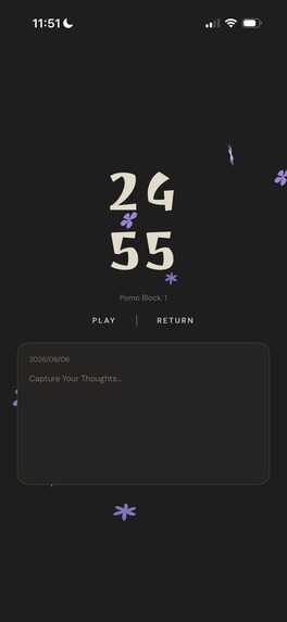
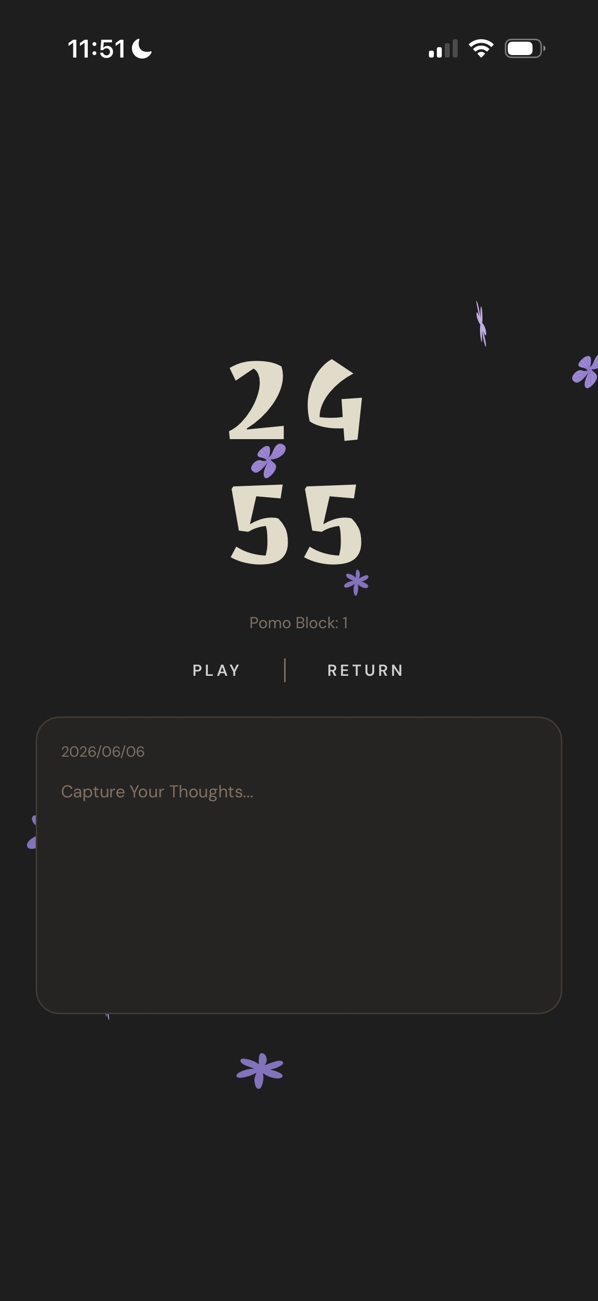
journal in focus session
-
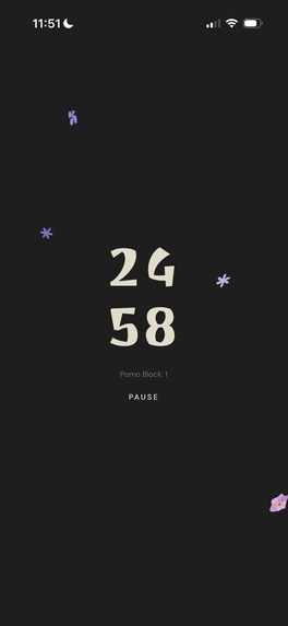
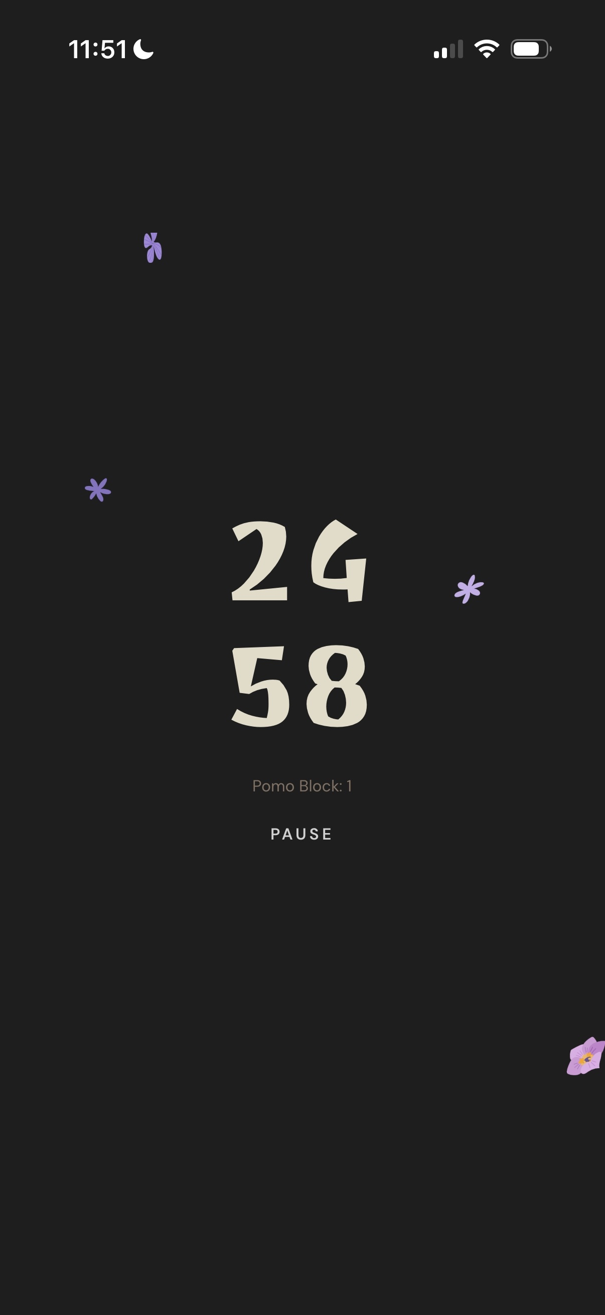
focus session
-

inner cluster
-

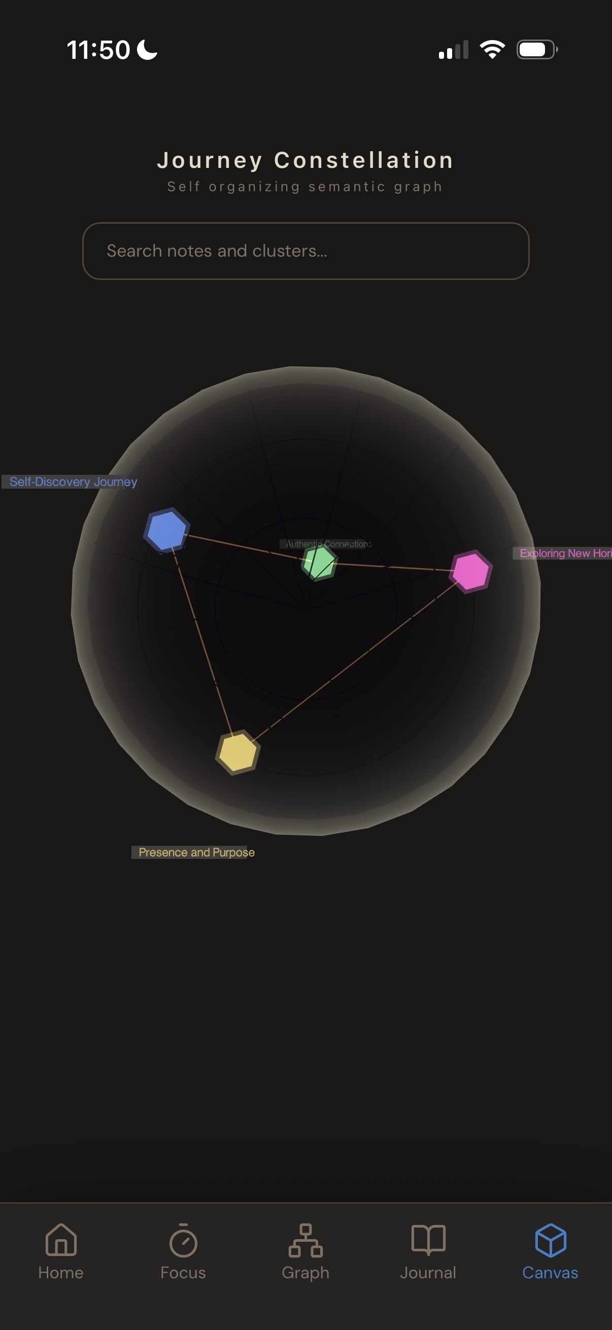
3d map
-

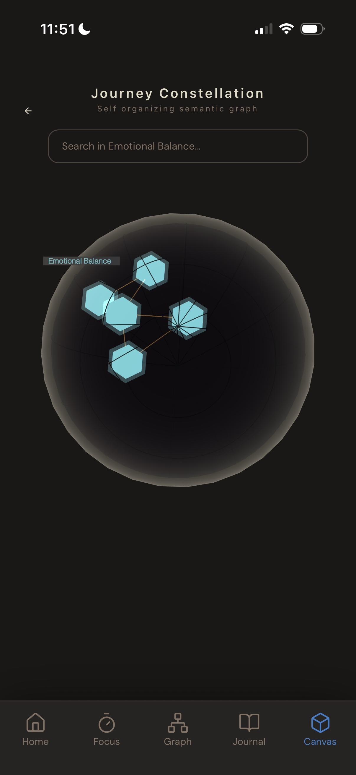
3d inner cluster
-
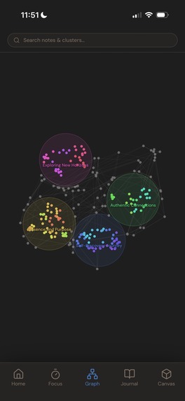
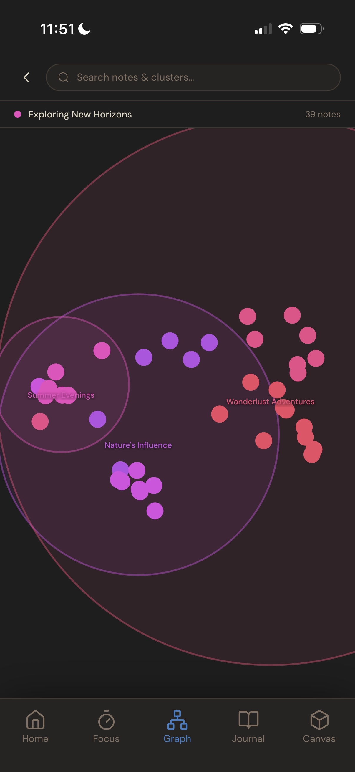
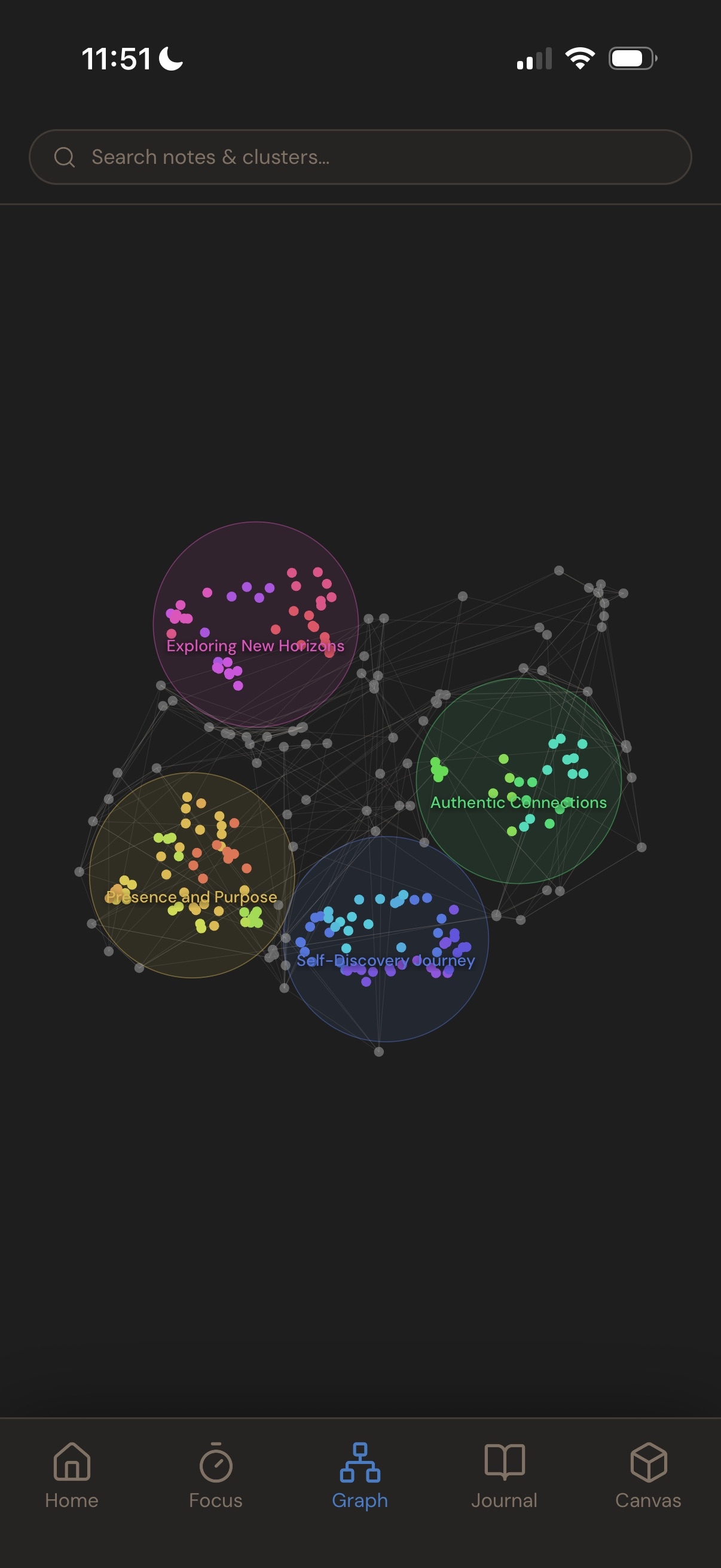
2d map
Daki Life: A Living Knowledge Graph for Your Mind
Problem Statement
Journaling is one of the most evidence-backed practices for mental clarity and personal growth, yet most people abandon the habit because it's inconvenient to maintain and trace back. It requires carving out dedicated time, staring at a blank page, and knowing what to say. And even then, each entry exists in isolation from what came before, making it difficult to spot patterns, connect ideas, and see how much you’ve actually grown.
Daki-Life makes journaling as convenient as possible while connecting all of your past ideas together. The main idea: journaling after a focus session during breaktime. If any idea crosses your mind, you can jot it down instantly. Over time, your notes self-organize into clusters (categories) with subtopics nested inside. Your ideas don’t disappear. They find each other
What It Does
Daki Life is a focus journal that builds a living semantic knowledge graph from your reflection notes.
- Focus: Pomodoro-style timer.
- Graph: Semantic Knowledge Graph. An interactive graph that automatically maps your notes into clustered life themes like Health, Creativity, and Relationships.
- Home: At-a-glance stats: sessions logged, top clusters by volume, and time-tracked categories.
- Day Summaries: List of days and the journals for that day
- Canvas: 3D representation of 2D graph.
The Algorithm Stack
Embedding
Notes are embedded at write-time via text-embedding-3-small (1536 dimensions) and stored in Supabase + pgvector. No retrieval-time re-embedding, every note already lives in semantic space.
Dimensionality Reduction: UMAP + PaCMAP
At each level of the cluster tree, two independent passes run on the raw 1536D embeddings in parallel:
UMAP 1536D → 8D: density-aware reduction whose output feeds directly into HDBSCAN. Parameters: metric=cosine, min_dist=0.0, densmap=True, n_epochs=500. Never used for visual layout.
PaCMAP 1536D → 2D / 3D: non-linear layout for the graph. Runs independently per cluster node so each tile has a locally coherent arrangement of its own notes. Tile positions are then computed globally by running PaCMAP on cluster semantic centroids and scaling each tile to fit without overlapping its neighbours.
UMAP is preferred over t-SNE for the clustering pass because it preserves global manifold structure: semantically related clusters remain near each other in the reduced space, not just internally tight.
HDBSCAN: Recursive Hierarchical Clustering
HDBSCAN runs recursively on the 8D output to produce a multi-depth cluster tree:
Root  ("Life")
  ├── Health
  │     ├── Running
  │     └── Sleep
  ├── Creativity
  └── Relationships
        └── Deep Connection
min_cluster_size adapts by depth:
$$k_{\min} = \begin{cases} \max(10,\; \lfloor n/16 \rfloor) & \text{depth} = 0 \ 3 & \text{depth} > 0 \end{cases}$$
Outlier notes (HDBSCAN label -1) are never force-assigned to the nearest cluster, they surface as standalone nodes at the depth where they first became noise.
Identity Persistence: Jaccard Matching
On every rebuild, new clusters are matched to old DB records via Jaccard similarity on note membership:
$$J(A, B) = \frac{|A \cap B|}{|A \cup B|}, \qquad \text{match if } J > 0.5$$
Labels are reused when a cluster's centroid hasn't drifted more than cosine distance 0.05, keeping your graph visually stable as new notes arrive.
Cosine Similarity Edges
$$\text{sim}(a, b) = \frac{a \cdot b}{|a|\,|b|}$$
Computed efficiently via L2-normalized matrix multiplication:
normed = embeddings / np.linalg.norm(embeddings, axis=1, keepdims=True)
sim_matrix = normed @ normed.T
Each note connects to its top-3 nearest neighbours within its leaf cluster. Cluster centroids connect to their top-3 sibling clusters to form the graph's backbone edges.
Cluster Metrics
Four scores are computed per cluster and min-max normalized across the full tree so they're always comparable regardless of corpus size.
Taxonomic Complexity: how much a cluster has structurally fractured into specific sub-thoughts. Instead of counting raw depth, it measures how deeply nested and populated the subtree is:
$$\text{TC} = \sum_{i \,\in\, \text{sub-clusters}} \bigl(\text{depth}_i \times \log(\text{note_count}_i)\bigr)$$
Information Density: vocabulary richness weighted by term specificity:
$$ID = \frac{U}{\sqrt{T}} \times \frac{1}{K} \sum_{k=1}^{K} w_k$$
where U = unique token types with non-zero TF-IDF weight, T = total raw word count, and w_1 through w_K are the top K TF-IDF scores (K = 8).
Semantic Cohesion: the mean cosine similarity of all note embeddings to the cluster centroid. High scores mean notes are tightly focused around a single idea:
$$Cohesion = \frac{1}{N} \sum_{i=1}^{N} \frac{v_i \cdot c}{|v_i| |c|}$$
Semantic Divergence: how distinct a cluster's thinking is from your overall baseline. Cosine distance between the cluster centroid c and the global centroid c_global (the average of every note in your database):
$$Divergence = 1 - \frac{c \cdot c_{global}}{|c| |c_{global}|}$$
A high divergence score signals niche interests or exploratory ideas far from your average thought.
All four scores are normalized to [0, 1]:
$$x_{norm} = \frac{x - min}{max - min}$$
Design Decisions
Tech Stack
- Mobile — React Native (Expo), TypeScript, Expo Router
- Graph rendering —
react-native-svg, D3 force simulation, Three.js - API — Node.js + Express
- ML sidecar — Python, FastAPI,
umap-learn,hdbscan,scikit-learn - LLM — OpenAI
gpt-4o-mini(labels),text-embedding-3-small(embeddings) - Database — Supabase (Postgres + pgvector + Auth + Realtime)
Roadmap
- Cross-user graph diffing: surface notes that are semantically close to another user's clusters (opt-in)
- Temporal drift tracking: visualize how your semantic clusters shift week over week
- Local-first storage: store notes and embeddings entirely on-device, eliminating the Supabase dependency for users who don't want their journal data leaving their phone
- On-device label generation: replace the GPT-4o-mini API call with a locally-run model (e.g. Phi-3 Mini or Gemma 2B via ONNX/llama.cpp) so cluster labels are generated without any note content transmitted to a third party
- Full offline mode: combine local storage and local label generation into a zero-cloud option, with opt-in sync for users who want cross-device access
Every note you write makes the graph smarter.
Built With
- expo.io
- hdbscan
- javascript
- node.js
- pacmap
- python
- react-native
- supabase
- typescript
- umap
- uvicorn

Log in or sign up for Devpost to join the conversation.