-
-
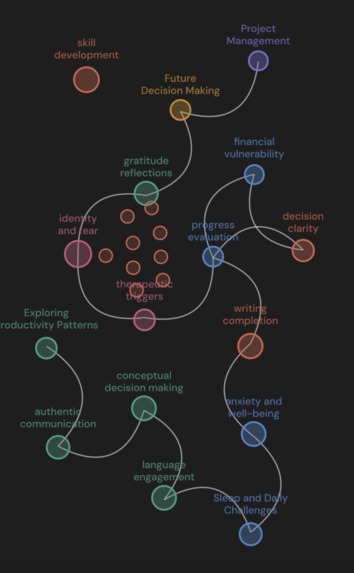
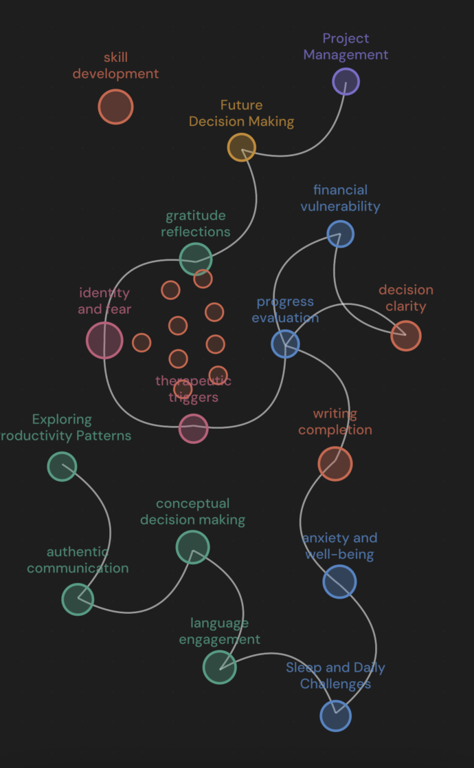
Semantic Graph
-
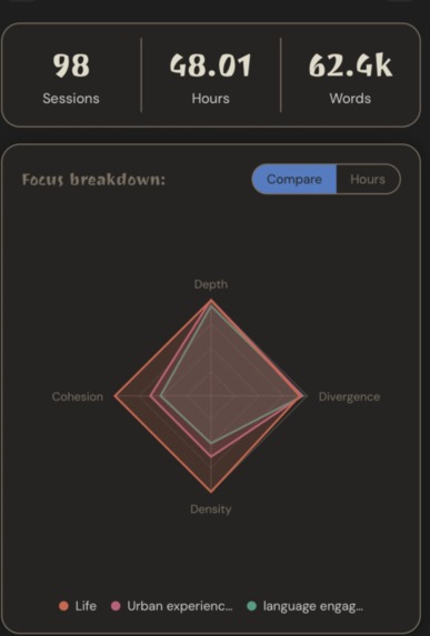
Spider Chart (metrics)
-
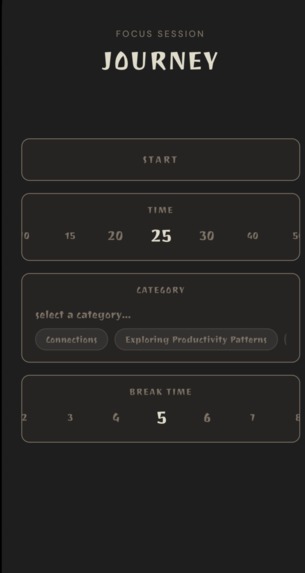
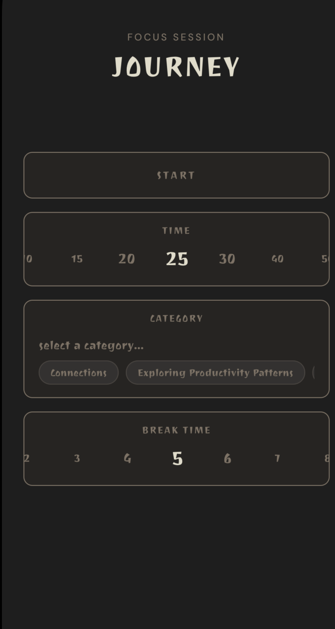
Focus Config

Daki Life — A Living Knowledge Graph for Your Mind
Problem Statement
Journaling is one of the most evidence-backed practices for mental clarity and personal growth, yet most people abandon the habit because it's inconvenient to maintain and trace back. It requires carving out dedicated time, staring at a blank page, and knowing what to say. And even then, each entry exists in isolation from what came before, making it difficult to spot patterns, connect ideas, and see how much you’ve actually grown.
Daki-Life makes journaling as convenient as possible while connecting all of your past ideas together. Two main ideas: journaling after a focus session during breaktime and journaling independently, either from a prompt or free writing. Over time, your notes self-organize into clusters (categories) with subtopics nested inside. Your ideas don’t disappear. They find each other
What It Does
Daki Life is a focus journal that builds a living semantic knowledge graph from your reflection notes.
- Focus — Pomodoro-style timer with structured reflection prompts at the end of each work block.
- Graph — Semantic Knowledge Graph — An interactive graph that automatically maps your notes into clustered life themes like Health, Creativity, and Relationships.
- Home — At-a-glance stats: sessions logged, top clusters by volume, and time-tracked categories.
Every note you write updates the graph in under 3 seconds for ~250 notes.
The Algorithm Stack
ClusterNode Object
The core of the backend operating on the ClusterNode object for the semantic journal graph
| Field | Type | Description |
|---|---|---|
id |
str |
Unique UUID for the ClusterNode |
parent_id |
Optional[str] |
ClusterNode parent (for traversing backwards) |
depth |
int |
Depth level of the ClusterNode |
note_ids |
list[str] |
All note IDs within the ClusterNode |
children |
list[ClusterNode] |
Children ClusterNodes (for traversing forwards) |
coordinates_2d |
dict[str, dict] |
2D coordinates for each note within the ClusterNode |
semantic_centroid |
Optional[np.ndarray] |
Each note's text content is given a 1536-dimensional vector; the semantic centroid is the average of all these vectors |
label |
Optional[str] |
All note texts undergo TF-IDF keyword extraction, producing a raw keyword list, which is then passed to a GPT-4o-mini API call to generate a label |
The ML pipeline is the product.
Embedding
Notes are embedded at write-time via text-embedding-3-small (1536 dimensions) and stored in Supabase + pgvector. No retrieval-time re-embedding — every note already lives in semantic space.
UMAP — Dimensionality Reduction
We run UMAP in two separate passes:
1536D → 8Dfor density-aware clustering (preserving local neighbourhood structure)1536D → 2Dfor graph layout (min_dist=0.1), so semantically similar notes appear physically close
UMAP is preferred over t-SNE because it preserves global structure across the full embedding manifold — clusters that are related stay near each other in 2D, not just internally tight.
HDBSCAN — Recursive Hierarchical Clustering
HDBSCAN runs recursively on the 8D output to produce a multi-depth cluster tree:
Root  ("Life")
  ├── Health
  │     ├── Running
  │     └── Sleep
  ├── Creativity
  └── Relationships
        └── Deep Connection
min_cluster_size adapts by depth:
$$k_{\min} = \begin{cases} \max(10,\; \lfloor n/16 \rfloor) & \text{depth} = 0 \ 3 & \text{depth} > 0 \end{cases}$$
Outlier notes (HDBSCAN label -1) are never force-assigned to the nearest cluster — they surface as standalone nodes at the depth where they first became noise.
C-TF-IDF — Discriminative Label Extraction
Each cluster is treated as a single document. C-TF-IDF surfaces words that are specific to a cluster — high within it, rare across siblings:
$$score(term, cluster) = tf(term, cluster) \times idf(term, all\ clusters)$$
$$where\ tf = 1 + \ln(count)$$ $$idf = \ln\left(\frac{1 + m}{1 + df}\right) + 1$$
Top-10 n-grams per cluster are passed to GPT-4o-mini for final 1–3 word human-readable labels.
Identity Persistence — Jaccard Matching
On every rebuild, new clusters are matched to old DB records via Jaccard similarity on note membership:
$$J(A, B) = \frac{|A \cap B|}{|A \cup B|}, \qquad \text{match if } J > 0.5$$
Labels are reused when a cluster's centroid hasn't drifted more than cosine distance 0.05 — keeping your graph visually stable as new notes arrive.
Cosine Similarity Edges
$$\text{sim}(a, b) = \frac{a \cdot b}{|a|\,|b|}$$
Computed efficiently via L2-normalized matrix multiplication:
normed = embeddings / np.linalg.norm(embeddings, axis=1, keepdims=True)
sim_matrix = normed @ normed.T
Each note connects to its top-3 nearest neighbours within its leaf cluster. Cluster centroids connect to their top-3 sibling clusters to form the graph's backbone edges.
Cluster Metrics
Four scores are computed per cluster and min-max normalized across the full tree so they're always comparable regardless of corpus size.
Taxonomic Complexity — how much a cluster has structurally fractured into specific sub-thoughts. Instead of counting raw depth, it measures how deeply nested and populated the subtree is:
$$\text{TC} = \sum_{i \,\in\, \text{sub-clusters}} \bigl(\text{depth}_i \times \log(\text{note_count}_i)\bigr)$$
Information Density — vocabulary richness weighted by term specificity:
$$ID = \frac{U}{\sqrt{T}} \times \frac{1}{K} \sum_{k=1}^{K} w_k$$
where U = unique token types with non-zero TF-IDF weight, T = total raw word count, and w_1 through w_K are the top K TF-IDF scores (K = 8).
Semantic Cohesion — the mean cosine similarity of all note embeddings to the cluster centroid. High scores mean notes are tightly focused around a single idea:
$$Cohesion = \frac{1}{N} \sum_{i=1}^{N} \frac{v_i \cdot c}{|v_i| |c|}$$
Semantic Divergence — how distinct a cluster's thinking is from your overall baseline. Cosine distance between the cluster centroid c and the global centroid c_global (the average of every note in your database):
$$Divergence = 1 - \frac{c \cdot c_{global}}{|c| |c_{global}|}$$
A high divergence score signals niche interests or exploratory ideas far from your average thought.
All four scores are normalized to [0, 1]:
$$x_{norm} = \frac{x - min}{max - min}$$
Design Decisions
| Problem | Algorithmic Choice | Why |
|---|---|---|
| Flat embeddings → spatial layout | UMAP (two-pass) | Faster than t-SNE; preserves global manifold structure |
| Finding themes without labels | HDBSCAN | Noise-robust; no need to pre-specify $k$ |
| Cluster labels that generalize | C-TF-IDF + GPT-4o-mini | Discriminative, not just frequent |
| Stable UX across rebuilds | Jaccard matching + centroid drift guard | Prevents graph thrashing on incremental updates |
| Graph layout performance | D3 force sim + UMAP 2D coords | Physics sim only for collision; semantic positions pre-computed |
The full rebuild runs: on cosine similarity, bounded by reducing the dimensions from 1536 to 8 before the heavy clustering passes. $$O(N^2 \cdot D)$$
Tech Stack
- Mobile — React Native (Expo), TypeScript, Expo Router
- Graph rendering —
react-native-svg, D3 force simulation - API — Node.js + Express
- ML sidecar — Python, FastAPI,
umap-learn,hdbscan,scikit-learn - LLM — OpenAI
gpt-4o-mini(labels),text-embedding-3-small(embeddings) - Database — Supabase (Postgres + pgvector + Auth + Realtime)
Roadmap
- Cross-user graph diffing — surface notes that are semantically close to another user's clusters (opt-in)
- Temporal drift tracking — visualize how your semantic clusters shift week over week
- On-device UMAP — eliminate the sidecar round-trip for small corpora using ONNX-exported models
Every note you write makes the graph smarter.
Built With
- expo.io
- hdbscan
- javascript
- openai
- python
- reactnative
- supabase
- typescript
- umap

Log in or sign up for Devpost to join the conversation.