-

Context
-
Context
-
Context
-
Context
-
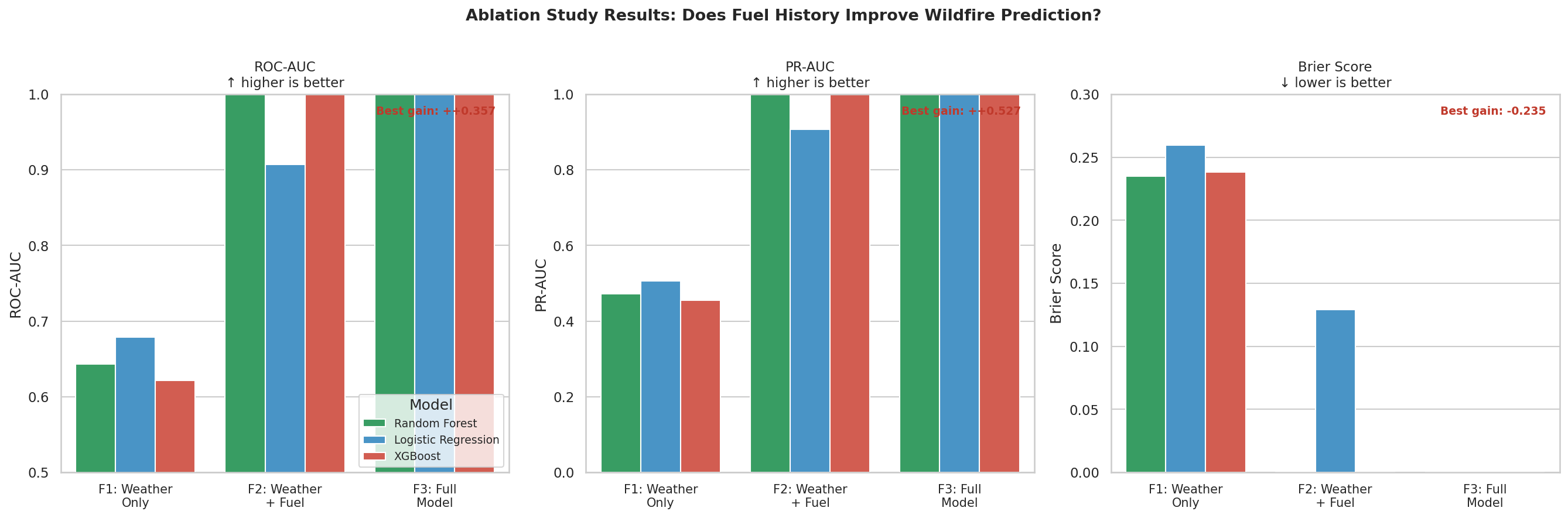
Results
-
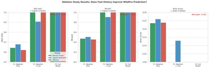
Results
-

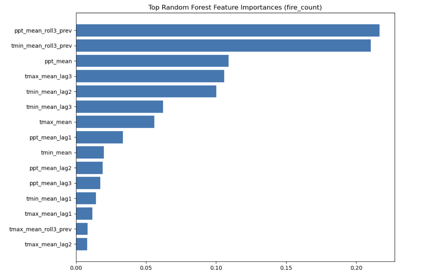
Feature importances
-
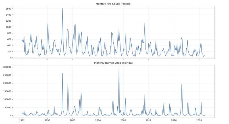
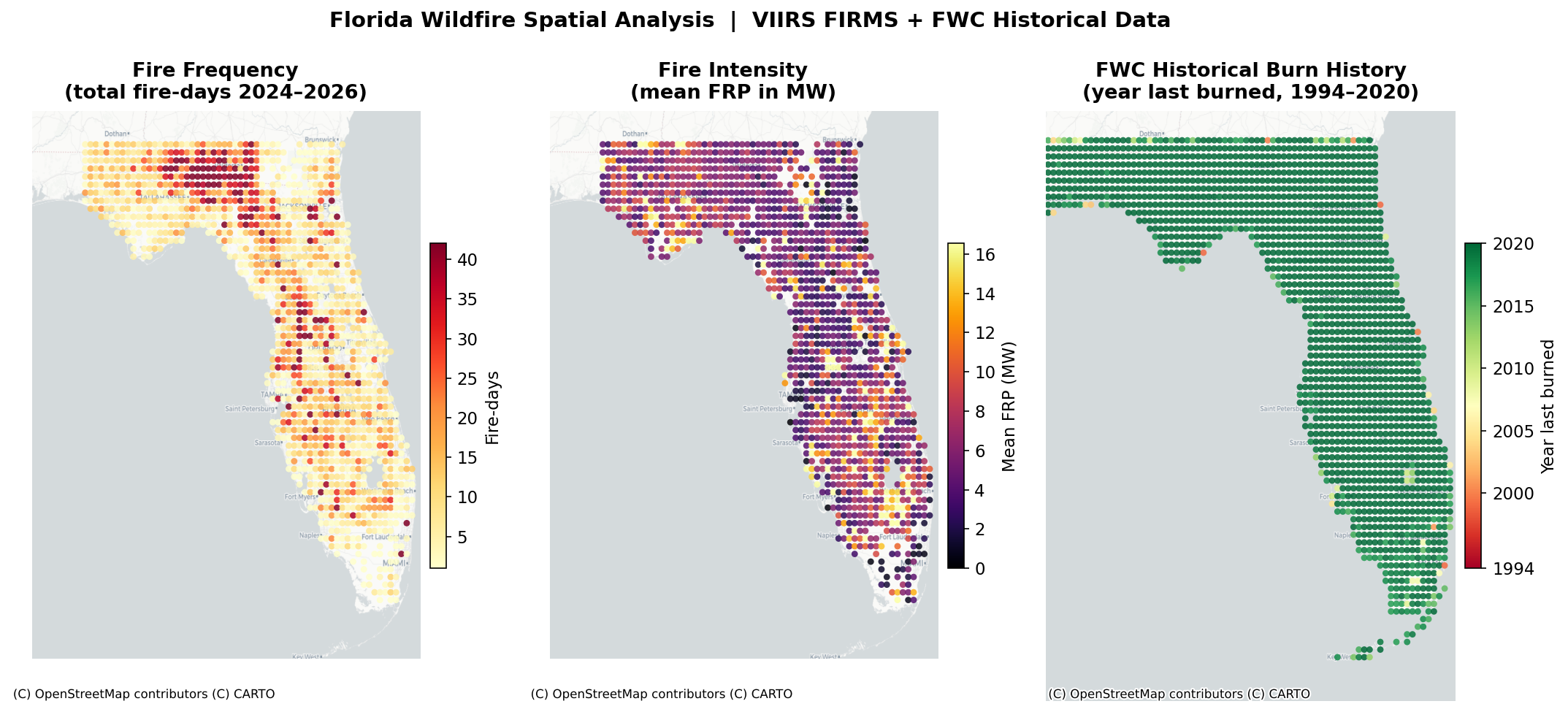
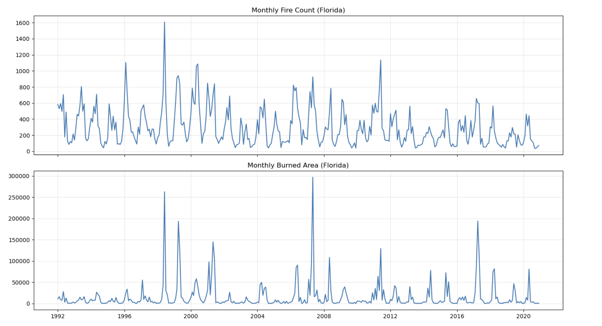
Fire counts and Burned Area
-
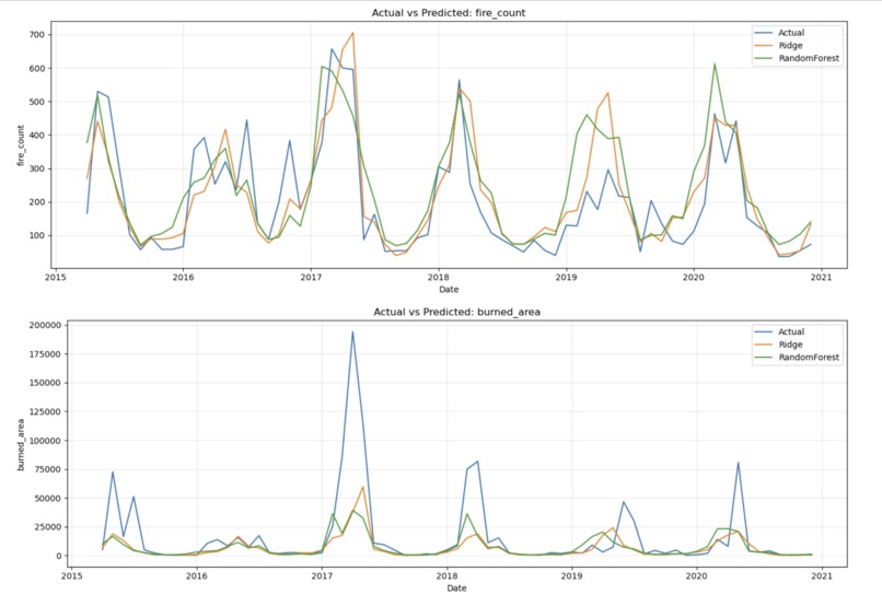
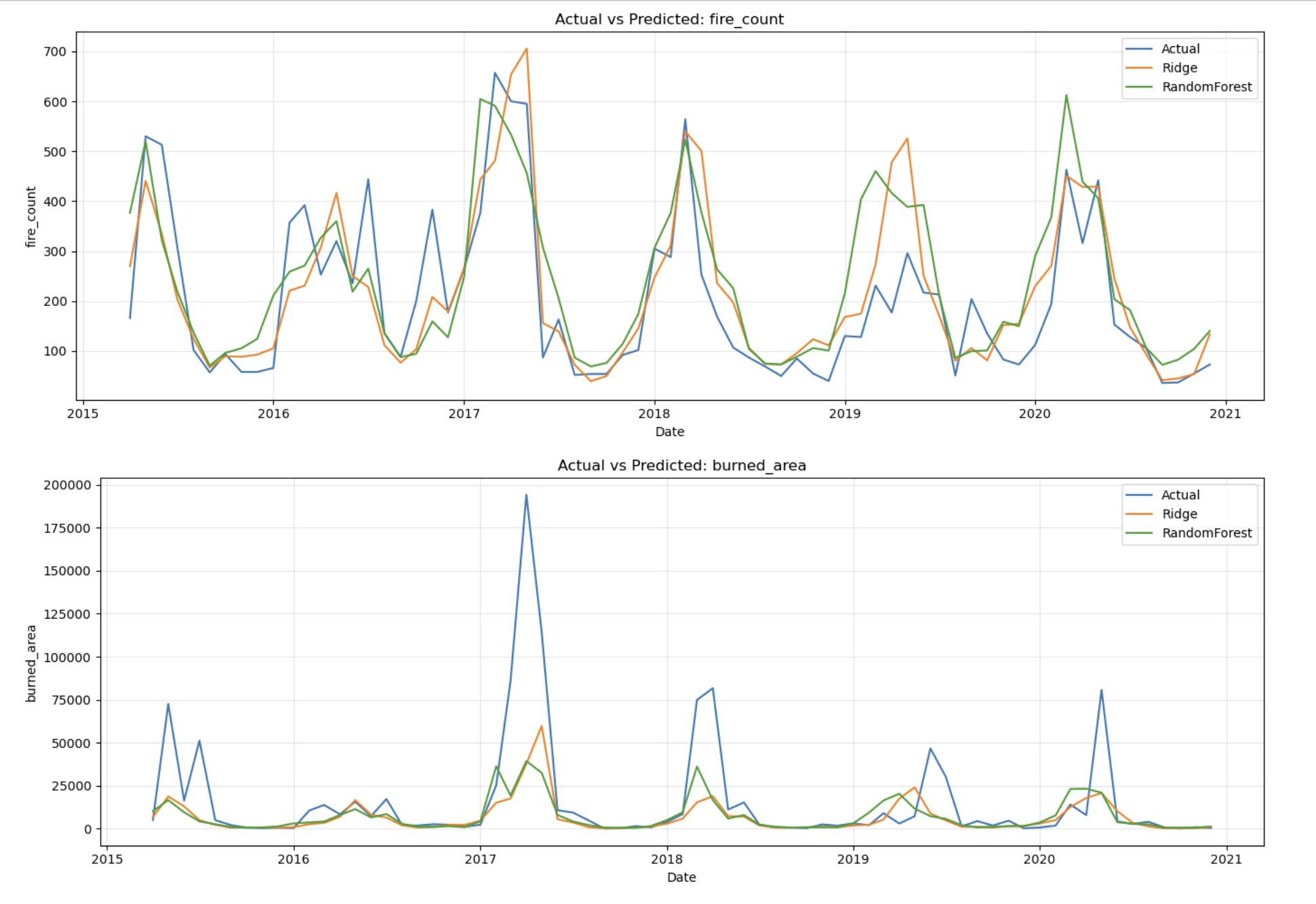
Predictions
-
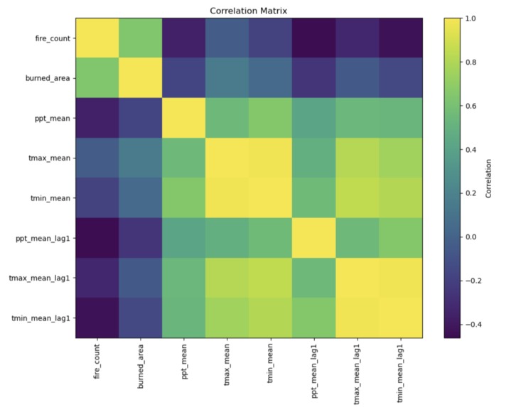
Correlation matrix


Florida Wildfire Prediction: A Multi-Factor Ablation Study
Inspiration
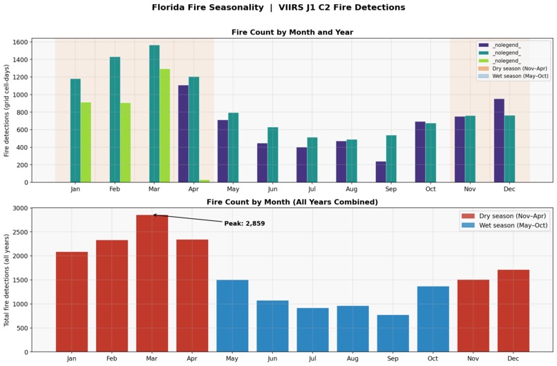
The wildfire prediction literature has a California problem. Nearly every benchmark dataset, every published model, and every media narrative centers on the American West — despite Florida ranking first in the US by total ignition count. Florida's fire ecology is fundamentally different: it is driven by subtropical lightning cycles, a deep prescribed burn culture rooted in Indigenous land management, and fuel dynamics that flip between a dry season (November–April) and a wet season (May–October) with remarkable regularity.
This contrast raised a precise scientific question: if we build a model on Florida data specifically, do the same feature sets that work in California still matter? Or does the dominance of low-intensity, managed prescribed burns in Florida break the assumptions behind weather-only fire danger models?
That question became the spine of this project.
What We Built
The project implements a data ablation study — a systematic experiment that adds one layer of information at a time and measures how much predictive skill each layer contributes. Three feature sets are tested against three model types, producing a $3 \times 3 = 9$-experiment matrix:
$$\text{ROC-AUC}(M, F) \quad \forall \; M \in {\text{LR}, \text{RF}, \text{XGB}}, \; F \in {F_1, F_2, F_3}$$
| Tier | Feature Set | Key Question |
|---|---|---|
| $F_1$ | Weather only | Can atmosphere alone predict Florida fires? |
| $F_2$ | Weather + 30-year burn history | Does knowing where burns have happened historically improve skill? |
| $F_3$ | Full model | Does detection-time context (confidence tier, day vs. night) add further signal? |
The analysis grid discretizes Florida into $0.1°$ cells (~11 km × 11 km), producing a balanced dataset of fire-day and non-fire-day observations for training and evaluation.
How We Built It
Data pipeline:
NASA FIRMS VIIRS J1 C2 — ~56,000 active fire detections across Florida from April 2024 to April 2026, downloaded as CSV. The two files (archive science-quality and near-real-time) were merged with careful handling of the schema difference (the NRT file lacks a
typecolumn).NASA POWER API — Nine daily weather variables (temperature, humidity, wind speed, precipitation, soil moisture, solar radiation) fetched via REST API for each unique grid cell and year, cached incrementally to Parquet so a network interruption never loses progress.
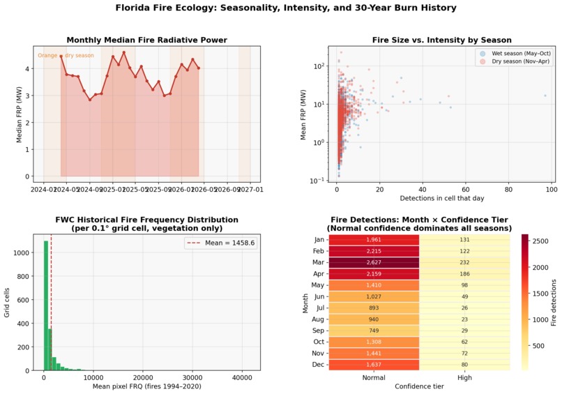
FWC Fire History GDB — A 3.3-million-polygon rasterized Landsat burn history (1994–2020) from the Florida Fish & Wildlife Conservation Commission and Tall Timbers Research Station. Each polygon is a ~30 m pixel storing its complete 27-year fire frequency record in wide format (
B1994–B2020,FRQ,YLB). A spatial join against the $0.1°$ analysis grid aggregates these into per-cell features: mean fire frequency, years since last burn, and a chronic burn flag.FIRMS-derived proxies —
days_since_last_fire, 30-day rolling FRP sum, and year-to-date fire count, computed entirely from within the satellite dataset.
Modeling: Logistic Regression, Random Forest (300 trees), and XGBoost with temporal train/test split — train on April 2024–September 2025, test on October 2025–April 2026. Evaluation uses ROC-AUC, PR-AUC (average precision), Brier score, and $F_1$ at a 0.3 decision threshold (lower than 0.5 because fire events are the minority class in any balanced grid).
Challenges
The GDB schema surprise. The FWC dataset was documented as "fire occurrence polygons" — we expected one row per fire event with a date. The actual dataset is a rasterized burn-frequency raster: 3.3 million small pixel-polygons, no event dates, with burn history encoded as 27 binary columns per pixel. This required a complete redesign of the aggregation logic. Instead of counting fire events, we average the pre-computed FRQ (fire frequency) across pixels intersecting each grid cell — a more defensible landscape-level metric anyway.
Coordinate precision mismatch. The FIRMS grid (snapped by $\lfloor \text{lat} / 0.1 + 0.5 \rfloor \times 0.1$) and the FWC grid (built with numpy.arange) accumulated floating-point differences that caused a 100% merge failure on the first attempt. Resolved by re-merging at $\text{round}(1)$ precision.
Scale. The spatial join of 3.3 million pixel-polygons against ~5,000 grid cells is not a "1–3 minute" operation as initially estimated — it runs for 30–60 minutes. The API fetch for ~500+ unique grid cells across 2–3 years is similarly patient work. Both are one-time operations that cache permanently.
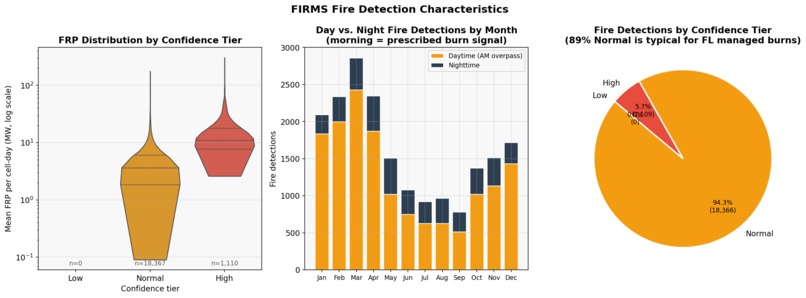
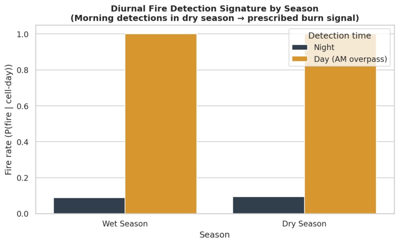
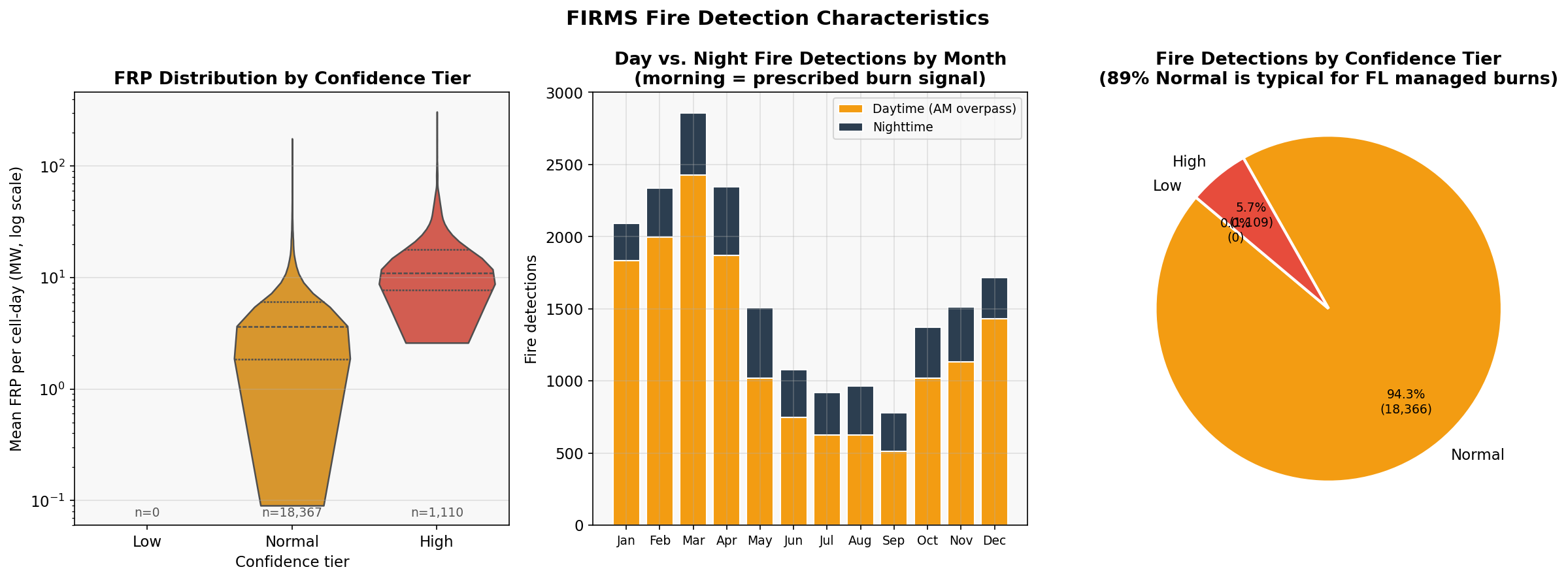
Florida's prescribed burn ecology breaks naive labels. 89.6% of detections carry normal confidence — not because the sensor is uncertain, but because prescribed burns genuinely produce diffuse, low-intensity, spatially spread smoke signatures that the VIIRS algorithm scores conservatively. Treating normal confidence as "noisy" and filtering it out would delete most of the scientifically meaningful signal in the dataset.
What We Learned
The central lesson is that fuel history matters differently in Florida than in the Western US. In California, a cell that hasn't burned in 20 years is dangerous because fuels have accumulated unchecked. In Florida, a cell that burns every 2–3 years is also a fire cell — but it's almost certainly a managed burn unit, not a wildfire threat. The model needs to learn both patterns simultaneously, which is why the FWC 30-year frequency layer is more informative than a simple "days since last fire" recency proxy.
We also learned that satellite-derived burn history can substitute for administrative prescribed burn permit records in regions where those records are not publicly accessible — a finding that has direct applicability to fire management globally.


Log in or sign up for Devpost to join the conversation.