• 

CohortScope: can a model tell a Rembrandt from a Rembrandt pupil?

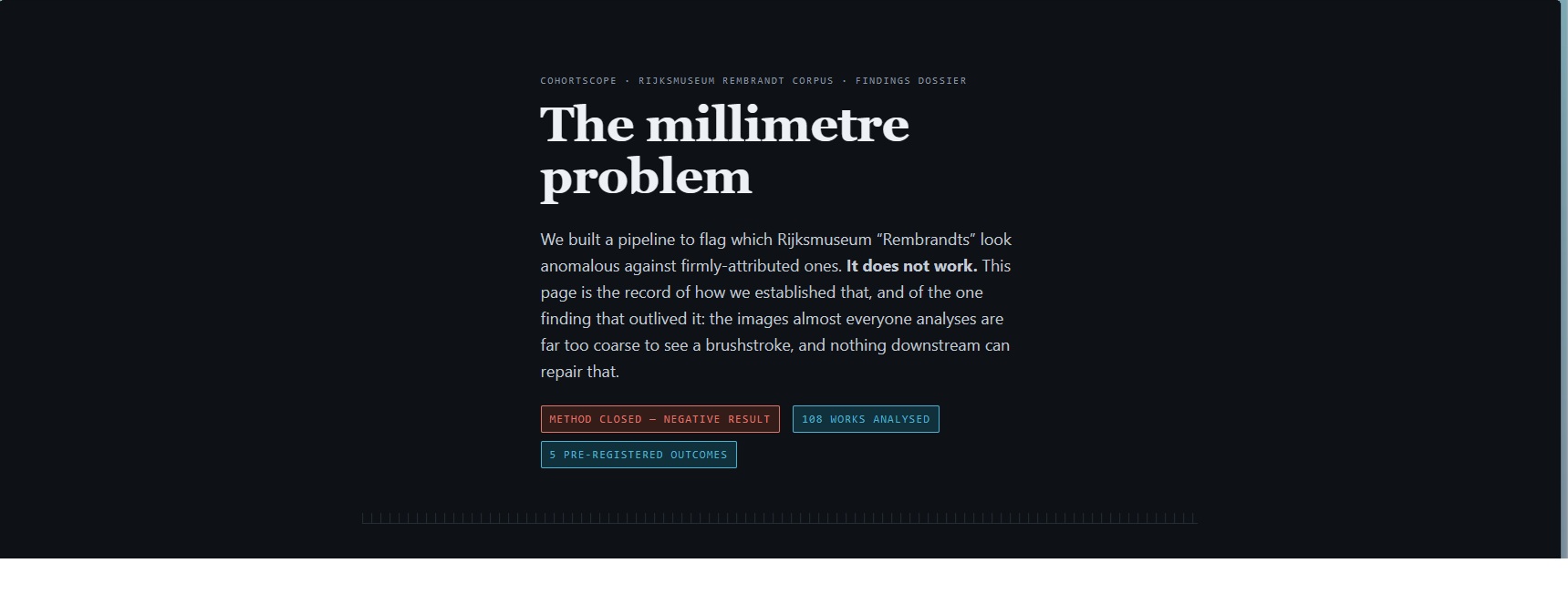
Report date: 2026-08-23 Repository: https://github.com/JialaiYing/CohortScope Findings page: results/dossier/index.html Answer: No, and we can say precisely why not.

---

1. Summary

CohortScope ranks Rijksmuseum Rembrandt oil paintings by how visually anomalous they look against a cohort of firmly attributed works, using a pretrained ResNet50 embedding (Signal A) and eight handcrafted texture and colour statistics (Signal B). The idea was that works by pupils and workshop members should score as outliers, giving curators a cheap triage list before expensive physical examination.

It does not work. Five pre-registered held-out tests:

Test	Question	Works ranked	AUC	Verdict
O04	Does one circle/workshop work clear the cohort 95th percentile?	1	n/a	weak
O06	Does the ranking separate 67 documented Rembrandt pupils?	90	0.419	fail
O09	Does Signal B work once every pixel means 0.20 mm of canvas?	55	0.469	fail
O11	Does Signal A work at 0.20 mm/px with no resize and no crop?	52	0.523	fail
O13	Was 0.20 mm/px simply the wrong scale? Sweep 0.15 to 0.30.	40 and 35	0.453 to 0.530	fail

Chance is 0.500. Every one of the eight sweep points sits within 0.047 of chance, and none clears even an uncorrected 95% confidence bar, let alone the Bonferroni-corrected bar the design locked in advance.

The finding that does hold up is the reason. In all four pupil tests, a single column of acquisition metadata separated the two classes better than the entire pipeline did:

Test	Pipeline AUC	Metadata column	Its AUC
O06	0.419	mm_per_px_analyzed	0.590
O09	0.469	mm_per_px_native	0.689
O11	0.523	mm_per_px_native	0.705
O13	0.530 (best of 8)	mm_per_px_native	0.617

Millimetres of canvas per pixel is a property of how the museum photographed the object, not of how the artist painted it. Whatever weak structure the model was picking up, it was closer to camera setup than to brushwork. That diagnosis is what produced the one genuinely reusable artifact in the project: a per-work verdict on whether a given painting can be analysed from published imagery at all.

---

2. The question, and why it is harder than it looks

Museums publish open, high-resolution images and rich metadata, but they have no cheap, explainable way to flag which works in an attribution group might merit re-examination. CohortScope narrows that to one museum and one artist:

Relative to Rijksmuseum oils currently attributed to Rembrandt van Rijn, which works look statistically unusual, and which measurable signal drove the flag?

The attribution literature says the discriminating evidence is largely in the handling: stroke width, loading, directional consistency, the physical trace of the hand. A seventeenth-century brushstroke is roughly 0.3 to 3 mm wide. That number turns out to be the whole story, and the project did not know it at the start.

The trap is that image files hide it. A 1500 px wide JPEG looks like a 1500 px wide JPEG whether the painting is a 15 cm panel or a 4 m canvas. The pixels are commensurable; the things they depict are not. Standard practice, resize the short edge to 256 and centre crop to 224, silently makes the problem worse, and does so differently for every object. Nothing in a normal CV pipeline surfaces this, and no accuracy metric distinguishes "the model cannot separate these classes" from "the model was never shown the evidence".

---

3. Methodology

3.1 Data

Rijksmuseum open collection API, no key required. Filters locked in config.py and never changed after the first harvest: type=painting, material=oil paint, imageAvailable=true. Images arrive over IIIF.

108 scored works. Splits are assigned by priority rules in acquire.py from catalogue text, not by hand:

Split	N	Rule	Role
cohort	23	firmly attributed to Rembrandt	fits the statistical normals; negative class
validation	1	title or attribution contains circle / workshop / school	held out for O04
ambiguous	1	"attributed to"	scored, never fitted, never counted
pupil (Tier 1)	67	creator matches a documented pupil roster	positive class for O06 onward
pupil (Tier 2)	16	associates rather than documented pupils	sensitivity only, never pooled

Four works on the pre-registered pupil roster did not make it in. Three (SK-C-371, SK-C-1598, SK-A-1627) were already claimed as excluded/other_artist by a Phase 1 probe, and the pre-registration forbids re-splitting a claimed work. One (SK-A-4034) returned IIIF 400 and failed closed. Reading the rule literally cost three usable samples. Amending it after seeing which three would have been a post-hoc edit to a pre-registered rule, so it was not done, and the loss is in the report instead.

3.2 Pipeline

Stages are flat modules at the repository root and run in order. Each has a frozen RECIPE_ID that names its output directory and is written into a manifest.json. Downstream stages assert the upstream recipe ID and take their worklist from that manifest, never from a filesystem glob or a fresh SQLite query.

acquire        Search API, Linked Art, IIIF   → SQLite + JPEGs
preprocess     two disjoint branches          → RGB PNG (branch H) and 224 tensors (branch C)
embed          ResNet50, penultimate layer    → 2048-d vectors
features       8 handcrafted scalars          → CSV
score          cohort normals, LOO            → ranked table + O04

The two preprocessing branches never cross. Branch H is EXIF-corrected identity RGB and its only consumer is features.py. Branch C is resized, cropped and ImageNet-normalised and its only consumer is embed.py. Handcrafted features are therefore never computed on tensors that a CNN transform has already distorted.

3.3 The two signals

Signal A, the embedding channel: cosine distance from a work's L2-normalised ResNet50 embedding to the cohort centroid, converted to z_A.

Signal B, the interpretable channel: eight scalars chosen to be readable by a human rather than to maximise anything. grad_mag_mean, grad_mag_std, grad_orient_entropy, laplacian_var, lbp_entropy, glcm_contrast, lab_chroma_mean, hue_circ_std. Each is z-scored against the cohort and z_B is the RMS of the eight.

combined = z_A + z_B. There is deliberately no learned weighting between them and no single opaque score: every row keeps its per-signal values and its named top drivers, so a flag can always be read as "flagged because of gradient magnitude variance", not just "flagged".

3.4 Fit rules

Normals are fitted on split=cohort only. Cohort works are scored leave one out: the centroid and the mean/standard deviation used to score work i are computed from the other 22 cohort works, so no painting contributes to the distribution it is measured against. Validation, ambiguous and pupil works use the full-cohort statistics and never enter a fit.

This is enforced structurally rather than by convention. Every fit path in score.py branches on meta[oid]["split"] == "cohort", so a split added later is non-fitting by construction and cannot leak in by someone forgetting to filter.

3.5 Evaluation protocol

Held-out separation is measured as ROC AUC between cohort (negative) and Tier 1 pupils (positive), equivalent to a Mann-Whitney U with tie handling. Confidence intervals are stratified percentile bootstrap, 10,000 resamples, with the seed written into the design document before the data existed (20260819 for O06, 20260822 for O09, 20260823 for O11, 20260824 for O13). Precision@k is reported at k = 5, 10, 20 against the base rate, since a triage tool that scores below base rate is worse than a random shortlist.

Outcome tiers were fixed in advance: fail if the CI lower bound is at or below 0.50, pass if AUC is at or above 0.70, weak otherwise.

---

4. Results and analysis

4.1 O04, the first held-out check: weak

SK-A-3934 (Borstbeeld van een lachende jonge man), the only circle/workshop work in the corpus. combined = 0.2826, rank 10 of 25. Cohort median is -0.1168 and the pre-registered pass bar, cohort p95, is 2.1069. It clears the median and does not come close to p95, which is weak by the locked rule.

Read honestly, this is one sample. It is not recovery of a clear anomaly and it is not a soft pass. The embedding channel was essentially null (z_A = 0.023) and what little signal there was came from Signal B. The correct response to a weak at N=1 is more held-out data, which is what came next.

4.2 O06, the first real test: fail

Harvesting works by documented Rembrandt pupils raised held-out N from 1 to 67.

Quantity	Value
AUC (combined, 23 cohort vs 67 Tier 1)	0.4192
bootstrap 95% CI	[0.2686, 0.5775]
z_A alone	0.4270
z_B alone	0.5224

Both signals are at chance and the combination is below it. Precision@k sits under the base rate at every k, meaning the ranking would give a curator a worse shortlist than drawing at random. The pre-registered confound check then found that mm_per_px_analyzed alone separated the classes at AUC 0.590, better than the whole two-signal pipeline.

That last number is what turned the project from "the method failed" into "find out why". A confound that beats the model is not noise; it is a pointer.

4.3 The resolution audit: what the images actually carried

dimensions.py records catalogued canvas size (cm_width, cm_height), native IIIF pixel dimensions, analysed pixel dimensions, and the derived mm_per_px_native and mm_per_px_analyzed, for all 108 works. All columns are nullable on purpose: the museum does not catalogue a size for every object, and "unknown" has to stay distinguishable from "fine".

Stage	mm of canvas per pixel	works finer than 0.30 mm/px
native IIIF, as published	0.015 to 0.812	85 / 108
analysed derivative (features_v1)	0.100 to 3.467	19 / 108
CNN input (embed_v1)	0.586 to 16.058	0 / 108

Three things fall out of this table.

Not one painting reached brushstroke scale at the CNN. Zero of 108. Signal A scoring 0.427 was never a fair test of the embedding; it was a test of an embedding that had never been shown the evidence.

The analysed corpus varied 35-fold in physical scale. Two works with identical pixel dimensions could differ by more than an order of magnitude in what a pixel covered. Any texture statistic computed across that corpus was comparing incommensurable quantities.

Only 6.3% of the published resolution was ever downloaded. The information was sitting on the museum's server the whole time. This is not a museum problem, it is a pipeline problem, and it is almost certainly not unique to this project.

4.4 Removing the confound: fetch area, not pixels

IIIF serves arbitrary regions at arbitrary sizes, so a patch of known physical size can be requested directly without downloading a gigapixel file. tiles.py takes 20 tiles per painting, each covering 30 mm × 30 mm of canvas delivered at 150 × 150 px. Every tile is 0.20 mm/px, on a 15 cm panel and on a 4 m canvas alike. Tile positions are evenly spaced over the row-major grid with no RNG, so the same database yields the same tiles every run.

The floor is a real constraint. A painting whose native resolution is coarser than 0.20 mm/px cannot supply the tile, and asking IIIF for it anyway would make the server upsample, inventing detail that was never photographed. Those works are reported as below floor and not scored. 64 of 108 works clear the floor; 44 do not, including six of the physically largest firm Rembrandts and the Night Watch at 0.310 mm/px native. The cohort drops from 23 to 17.

Losing the Night Watch to your own eligibility rule is uncomfortable, and it is the correct behaviour. Scoring it on inadequate pixels would produce a number, and the number would be meaningless.

4.5 O09, Signal B on commensurable pixels: fail

tile_features.py calls the same features.extract_one() with the same constants as features_v1. The only difference between the two arms is what a pixel means, which is the experimental control.

Arm	pixels	AUC
tile_scores_v1	0.20 mm/px everywhere	0.469
features_v1 re-fit on the same 55 works	fixed 1500 px wide, 0.100 to 0.947 mm/px	0.427
ΔAUC		+0.042, 95% CI [-0.141, +0.223]

The baseline is re-fitted from scratch on the same population rather than quoted from O06, so the two arms differ in exactly one thing. Physical normalisation moved the number by less than its own confidence interval. mm_per_px_native scored 0.689 on this population, again beating the pipeline.

One methodological note that looks like an edge case and is not. hue_circ_std is undefined on 77 near-grey tiles. Dropping those tiles would have been content-based filtering with a class-correlated rate (7 of 17 cohort works affected versus 11 of 38 Tier 1), which the design forbids. The rule written before any aggregate was computed: keep the tile, exclude that one cell from that one feature's median. This was decided and committed before the AUC existed, which is the only reason it is credible.

4.6 O11, Signal A on commensurable pixels: fail

The obstacle O09 named was that a 150 px tile cannot enter a 224 px backbone without a resample factor, which is exactly the arbitrariness the tiling exists to remove. The resolution is arithmetic, not a choice: 224 px (fixed by the backbone) × 0.20 mm/px (the locked floor) = 44.8 mm. The region arrives at the backbone's native input size, so tile_embed.py applies only ImageNet normalisation. No resize, no crop, no interpolation. It deliberately does not call the shared CNN transform, whose 256-resize and 224-crop are precisely what makes the analysed mm/px vary per work.

Arm	AUC
tile_scores_a_v1 (z_A_tile)	0.523
embed_v1 re-fit on the same 52 works	0.391
ΔAUC	+0.132, 95% CI [-0.092, +0.352]

This is the largest movement any change in the project produced, and it still means very little. The fixed-pixel arm was clearly below chance; commensurable pixels brought it back to chance. The interval contains zero. Precision@5 is 0.200 against a base rate of 0.692. mm_per_px_native scored 0.705, with Spearman rho of -0.422 against the score itself, which is the same confound firing harder.

The larger tile costs 3 works, and interestingly they are the physically smallest (SK-A-3982, SK-A-88, SK-A-89), whereas the D34 exclusions were the largest. The two tile recipes are size-biased in opposite directions. Because Signal A and Signal B now live on different populations (52 and 55 works), there is deliberately no combined score on either tile recipe. Summing z-scores across different corpora would be meaningless.

4.7 O13, the resolution sweep: fail

The last live hypothesis was that 0.20 mm/px was simply the wrong scale. sweep.py re-ran both signals at 0.15, 0.20, 0.25 and 0.30 mm/px, holding each signal's pixel count fixed so that only millimetres per pixel varied.

Signal B, 150 px tiles, 16 cohort vs 24 Tier 1, base rate 0.600:

floor	tile canvas	AUC	95% CI	corrected CI
0.15	22.5 mm	0.466	[0.286, 0.651]	[0.224, 0.716]
0.20	30 mm	0.474	[0.292, 0.656]	[0.224, 0.724]
0.25	37.5 mm	0.484	[0.286, 0.677]	[0.224, 0.750]
0.30	45 mm	0.495	[0.310, 0.682]	[0.242, 0.757]

Signal A, 224 px tiles, 15 cohort vs 20 Tier 1, base rate 0.571:

floor	tile canvas	AUC	95% CI	corrected CI
0.15	33.6 mm	0.453	[0.250, 0.667]	[0.170, 0.760]
0.20	44.8 mm	0.530	[0.310, 0.757]	[0.230, 0.838]
0.25	56 mm	0.503	[0.283, 0.720]	[0.197, 0.810]
0.30	67.2 mm	0.473	[0.263, 0.690]	[0.180, 0.773]

All eight corrected intervals contain 0.50, and so do all eight uncorrected ones. The multiplicity correction never had to do any work, because not a single point cleared even the unadjusted bar. Signal B spans 0.029 across a 2× change in resolution. The curves are flat, not noisy-but-trending.

Two design choices here are load-bearing and easy to get wrong.

The population is fixed across floors, not re-derived per floor. Eligibility is not monotonic in the floor: a coarser floor admits more works by the mm/px test but excludes more by the "20 tiles must fit on the canvas" test. Re-deriving the population per floor would confound resolution with which paintings entered the sample, and the resulting curve would be uninterpretable. Holding it fixed costs sample size (the 0.05 to 0.40 intersection is 6 works for Signal B and zero for Signal A, which is why the range is 0.15 to 0.30) and buys the only version of the experiment that answers the question asked.

Multiplicity is corrected, and corrected in advance. Four floors × two signals = 8 tests. Reading the best of eight against an uncorrected 95% interval inflates the false-positive rate to roughly 34%. The design locked a Bonferroni correction to a 99.375% interval before any point existed, and both intervals are computed from the same bootstrap draws at every point, so the correction cannot be applied selectively to a winner.

4.8 What the three escape hatches were, and how each closed

"It failed because..."	Test	Outcome
...N was too small	O06 raised held-out N from 1 to 67	got worse, 0.419
...the images were incommensurable	measured it: 35× spread, 0/108 at brushstroke scale	confound was real
...so fix the scale and it will work	O09 and O11 on 0.20 mm/px tiles	0.469 and 0.523
...0.20 was the wrong scale	O13 swept 0.15 to 0.30, population fixed	8 points, all at chance

Each row is a pre-registered experiment with a design document committed before its data existed. The question is closed. A sixth variant of the same method is not warranted without new evidence, and the imagery to test a finer hypothesis does not exist in this collection: nine works in the entire corpus have imagery finer than 0.05 mm/px, and zero support a full-range sweep for Signal A.

---

5. Reasoning behind the crucial decisions

The full log is docs/decisions.md, D01 through D38, each dated. Six decisions changed what the project could conclude.

D19 to D21, D32: splits come from catalogue text, not from judgement

Split assignment is a priority rule over description and creator fields in acquire.py. The alternative, deciding case by case which works "look like" workshop pieces, would have made the labels a function of the same visual intuition the model was supposed to test. Machine-readable provenance is a weaker label but an independent one.

The cost is visible: three pupil works were lost because a Phase 1 probe had already claimed them, and the rule forbids re-splitting. Keeping the rule and reporting the loss is the whole point of having the rule.

D30: leave-one-out cohort fits, enforced by control flow

With a cohort of 23, letting a work contribute to the normal it is scored against would pull its own z-score toward zero and make the cohort look artificially tight. LOO is standard; what is less standard is enforcing it structurally. Every fit path branches on the split, so a new split is non-fitting by construction. A convention someone has to remember is a leak waiting to happen.

D30, again: no single opaque score

combined = z_A + z_B with both components and the named top drivers kept on every row. A learned combination would have been trivially better on paper and would have needed a training set, which does not exist here at this N, and would have destroyed the ability to say why a work was flagged. For a triage tool whose users are curators, the explanation is the product. In hindsight this decision is what let the failure be diagnosed at all: because the signals were separable, O06 could report z_A = 0.427 and z_B = 0.522 independently, which is what pointed at the embedding branch first.

D33: capture geometry, change no score

dimensions.py records physical dimensions and derived mm/px, and features.py, embed.py and score.py do not read those columns. Resampling to a fixed physical resolution was a separate, still-unmade decision at that point, and the audit report deliberately declined to pick a floor. Mixing data capture with a scoring change would have made it impossible to attribute any subsequent difference to either one.

This is the decision that produced the diagnosis. It changed no number and it explained every number.

D34: fetch fixed physical area, and report the works you cannot answer

The obvious fix for incommensurable pixels is to resize everything to a common mm/px. That either upsamples (inventing detail) or downsamples the good images to match the bad ones. Requesting IIIF regions of fixed physical size avoids both, at the cost of a hard eligibility floor.

The floor is derived at query time and never stored on the works table. The table holds measured facts; the floor is policy; cached policy goes stale silently and nobody notices. That separation is why python tiles.py --plan can answer the eligibility question for a different floor without a migration.

D37: fix the population before sweeping, and correct for multiplicity in advance

Both discussed in §4.7. The short version: a sweep with a per-floor population answers a different and less interesting question, and eight uncorrected tests will hand you a significant result about a third of the time whether or not one exists.

---

6. Evaluation of the model training process

6.1 There was no training, and that was a decision

No weights were updated at any point. Signal A uses ImageNet-pretrained ResNet50 as a frozen feature extractor; Signal B is closed-form image statistics. The "fitting" in this project is limited to computing a mean, a standard deviation and a centroid over 23 cohort works, leave one out.

That was the right call at this scale and it is worth being explicit about why. Finetuning on 23 positives with 67 held-out negatives would overfit long before it generalised, and any held-out score would then be a statement about the split rather than about Rembrandt. There is no honest train/validation/test partition to be had from 108 works, and a project whose entire credibility rests on pre-registration cannot afford a learned model whose behaviour depends on choices made after seeing data.

The consequence has to be stated with equal clarity: ImageNet features are not brushwork features. ResNet50 was trained to separate object categories, and the distinction between a Rembrandt and a Bol is not an object-category distinction. A flat Signal A curve is evidence against this embedding, not against learned representations in general.

6.2 What was actually validated, and how

Concern	How it was handled
Self-scoring / leakage	LOO centroid and LOO mean/std for cohort rows; enforced by control flow, not convention
Label leakage into fits	Only split=cohort fits; pupil and ambiguous never enter a normal
Threshold tuning after the fact	Every threshold, seed and k transcribed from a design document committed before acquisition
Multiple comparisons	Bonferroni correction locked in advance for the 8 sweep tests; both intervals printed at every point
Baseline gaming	Every ΔAUC re-fits the baseline from scratch on the same population, so only one thing differs between arms
Content-based filtering	A tile is never dropped for what it depicts; undefined feature cells are excluded per-feature
Silent failures	Each stage writes results/qc_<recipe_id>/ with a failures CSV and a summary JSON
Output drift	Frozen recipe IDs; stages refuse to overwrite without --force; verification is re-run and diff the manifest

A Phase 4 leakage and scope review (results/phase4_review.md) passed independently of the authors of the scoring code.

6.3 Where this evaluation is weak

Power. N is 40 and 35 in the sweep, 55 and 52 in O09 and O11. These are well powered for a large effect and badly powered for a small one. Failing to find an effect is not the same as showing there is none, and the confidence intervals in §4.7 are wide enough to admit a real AUC of 0.65 at some floors. The claim defended here is narrow: no effect large enough to be useful for triage was detectable under these conditions.

One museum, one artist, one backbone. Nothing here generalises to other collections without re-running it.

Tier 2 works were never pooled, by design, so the sensitivity analysis they were meant to support is thin at sweep scale (one work per sweep).

The negative result depends on the pupil labels being right. They come from museum creator fields matched against a documented pupil roster, which is better than guesswork and worse than scholarly consensus.

6.4 What a stronger claim would need

Higher native resolution than this collection publishes, for a start: raking-light or macro imagery at 0.05 mm/px or better, which exists for individual famous works and not for corpora. Beyond that, a representation trained on handling rather than on object categories, and a held-out set an order of magnitude larger with provenance-grade labels. Those are all real research programmes rather than a next sprint, and none of them is reachable by re-tuning what is in this repository.

---

7. What actually ships

The ranking is not usable and the repository says so in every report, in the demo viewer's own banner, and on the findings page. What is reusable is the adequacy verdict.

python tiles.py --plan

Runs offline in under a second against the committed SQLite database and reports, per work, whether the question can be answered from published imagery at the 0.20 mm/px floor and, when it cannot, which test it failed. 64 of 108 answerable, 44 not.

That verdict is independent of whether the ranking works, applies to any IIIF collection, and answers a question a curator or a digitisation team actually has: is our imagery good enough to support this kind of analysis, and if not, what would we need to re-photograph? For this corpus the honest answer for 44 works is no, and saying so is more useful than returning a confident-looking number computed from pixels that cannot support it.

---

8. Reproducing this

Everything except two regenerable caches is committed, so a clone reproduces the whole result without network access.

mamba activate CohortScope
python -m pip install -r requirements.txt

python preprocess.py       # rebuilds the ~340 MB cache byte-identically
python features.py --force
python score.py --force            # O04
python evaluate_pupils.py --force  # O06
python resolution_audit.py --force
python tile_score.py --force       # O09
python tile_score_a.py --force     # O11
python sweep.py --force            # O13
python dossier.py                  # the findings page

Tile stages need python tiles.py / python cnn_tiles.py / python sweep.py --fetch first if data/tiles/ is absent; those are the only steps that touch the network, along with acquire.py and dimensions.py. There is no test suite and no CI. Verification is by re-running a stage with --force and diffing its manifest against the committed one.

Artifact	Path
Findings page	results/dossier/index.html
Ranked scores and fit manifest	results/scores/
O04 / O06 / O09 / O11 / O13 reports	results/*_report.md
Pre-registrations, committed before their data	results/phase{4,7,8,9,10,11}_*_design.md
Decision log, D01 to D38	docs/decisions.md
Physical geometry	data/cohortscope.sqlite, works.mm_per_px_*
Per-recipe QC logs	results/qc_*/

---

9. Closing

The ranking does not work and should not be used. What the project produced instead is a measurement and a tool.

The measurement: on this corpus, model-based attribution triage is limited not by architecture and not by sample size but by how much canvas a published pixel covers. That quantity is recorded, auditable, and worse than most people assume. Only 6.3% of the resolution the museum already publishes was reaching the model, and after a standard resize-and-crop not one painting in 108 was being shown a brushstroke.

The tool: a per-work verdict on whether the question is answerable at all, derived from the museum's own IIIF metadata, that does not depend on the ranking being correct.

Five outcomes, five design documents committed before their data, no threshold edited after the fact. A negative result that is this specific about its own cause is a more useful contribution than a positive one nobody could reproduce.

Built With

• cv
• gradio
• python
• pytorch
• resnet50
• rijksmuseum
• scikit-learn
• sqlite