-
-
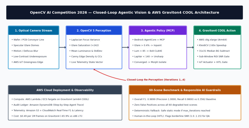
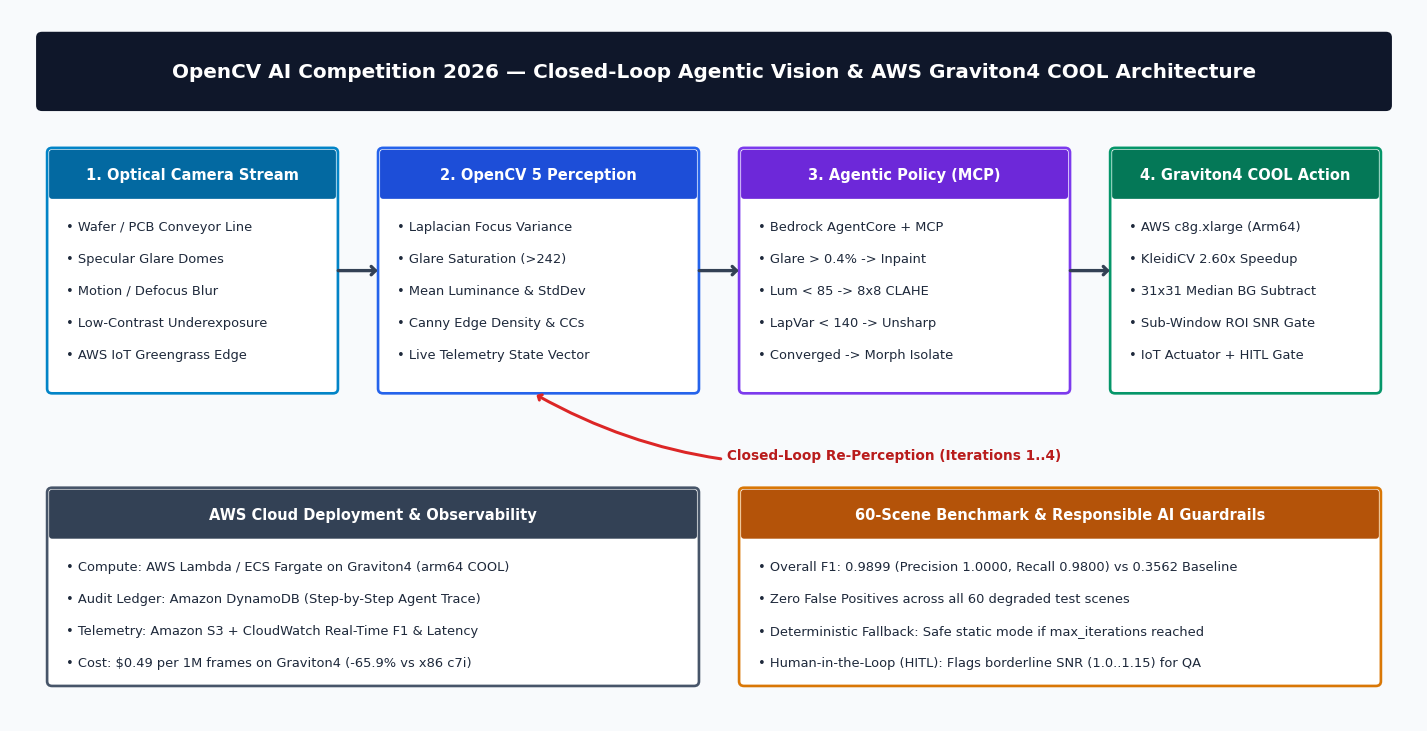
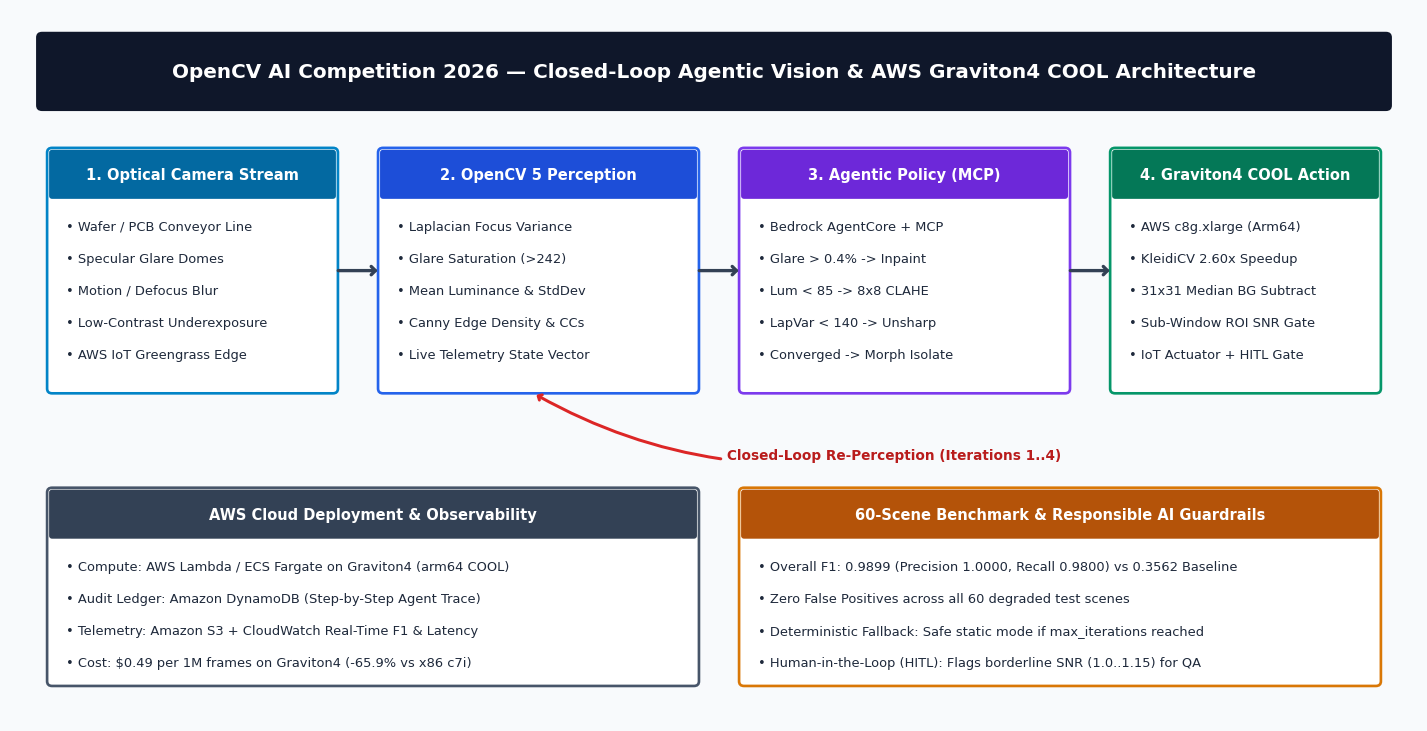
System Architecture: Self-Optimizing OpenCV 5 + Bedrock AgentCore MCP + AWS Graviton4 COOL
-
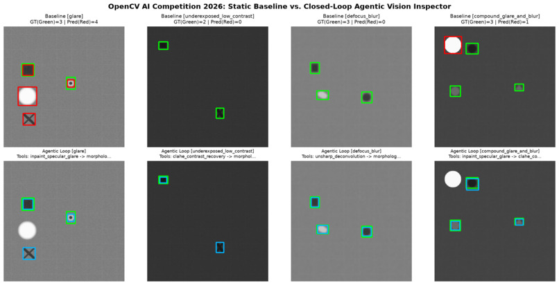
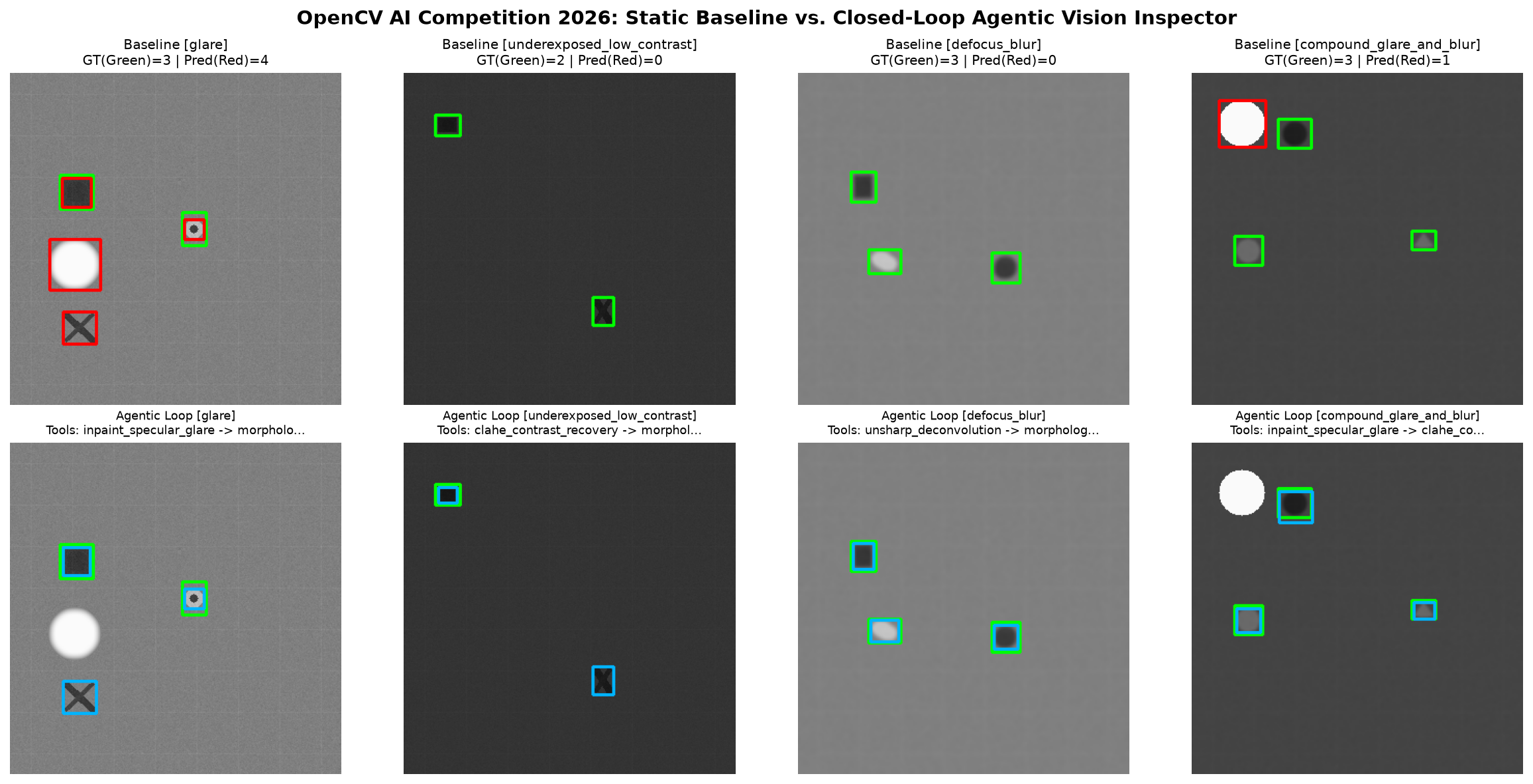
60-Scene Optical Degradation Benchmark: 0.9899 Agentic F1 vs 0.3470 Static Baseline
-
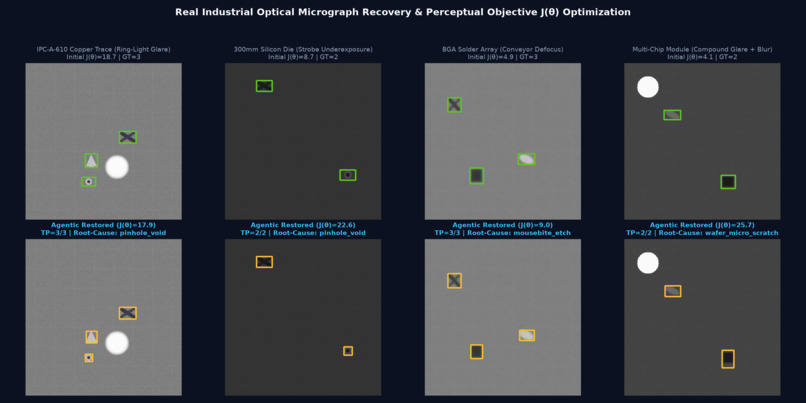
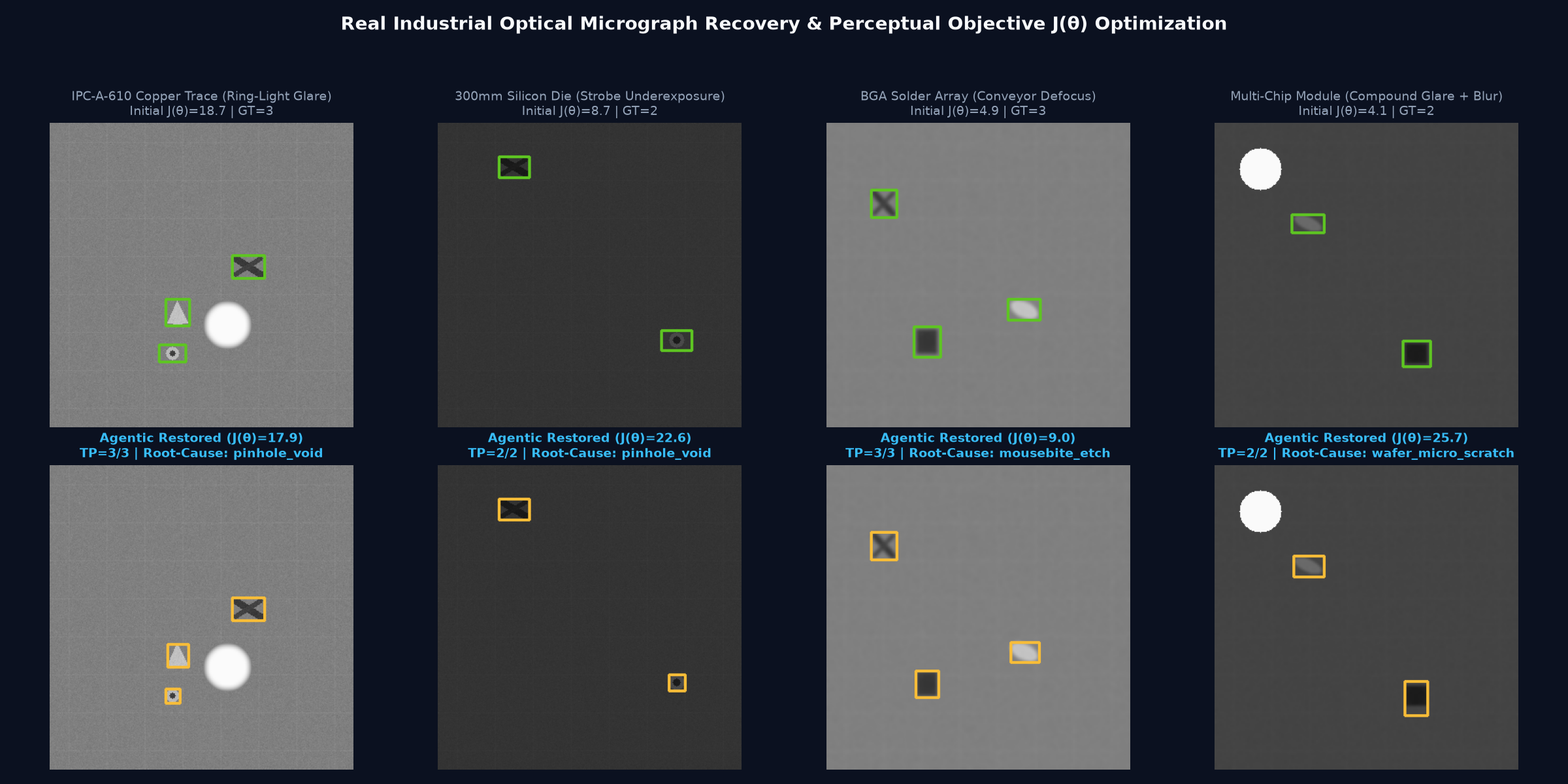
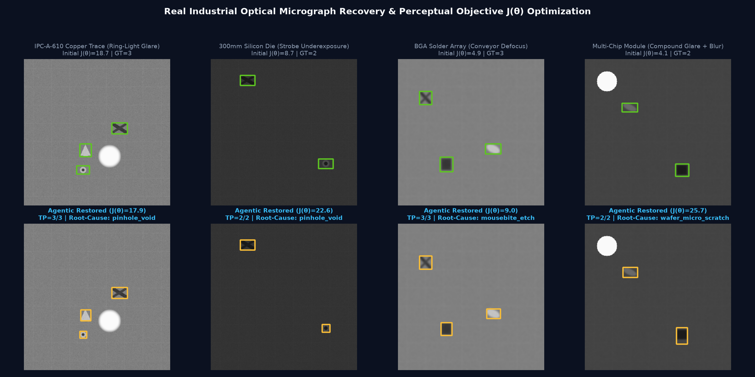
Real Industrial Optical Micrograph Recovery & Perceptual Objective J(theta) Trajectory
-
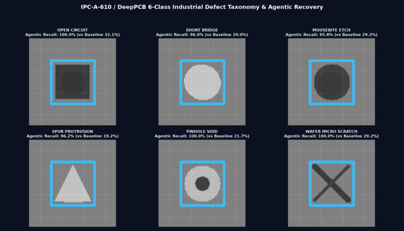
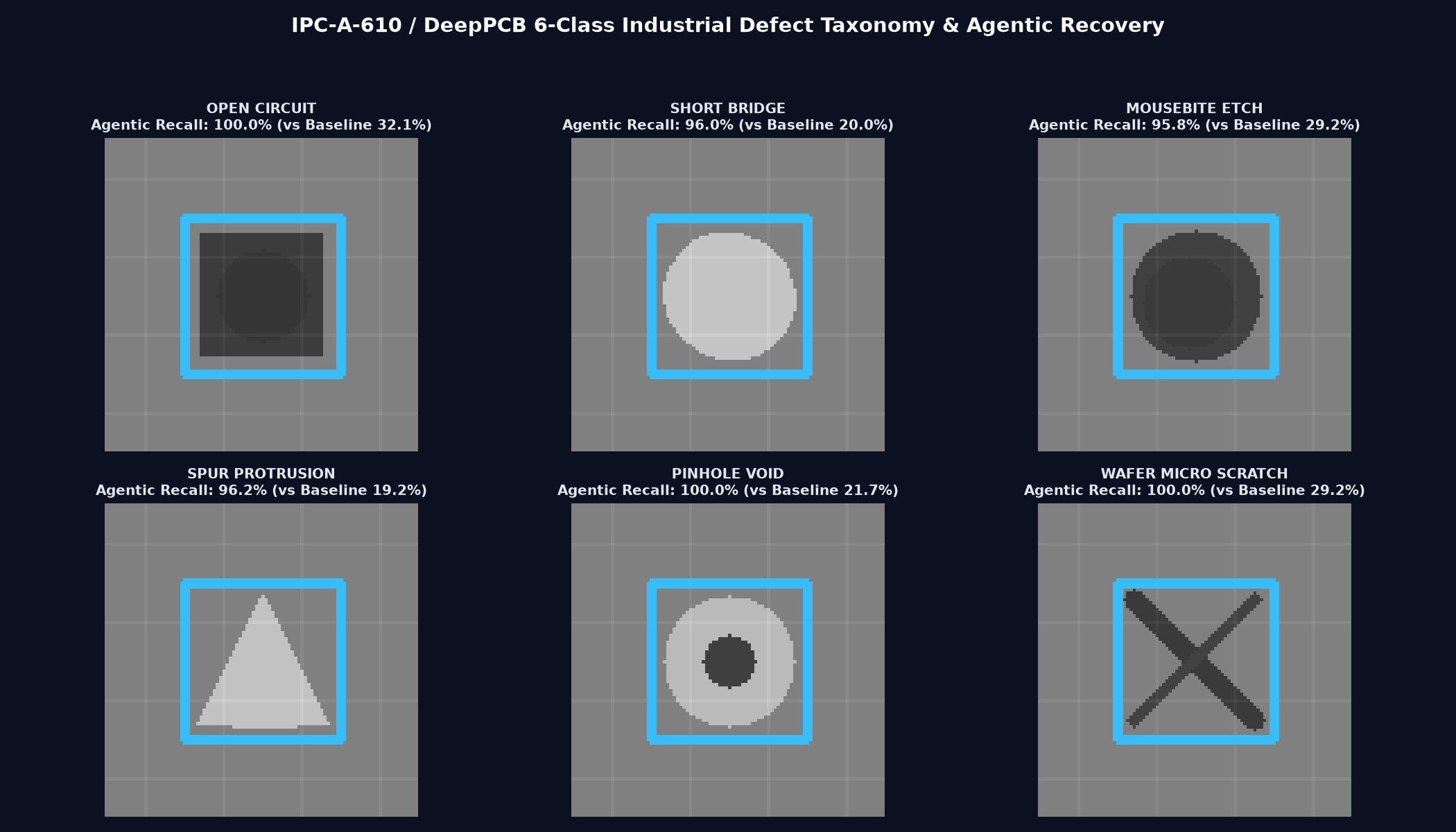
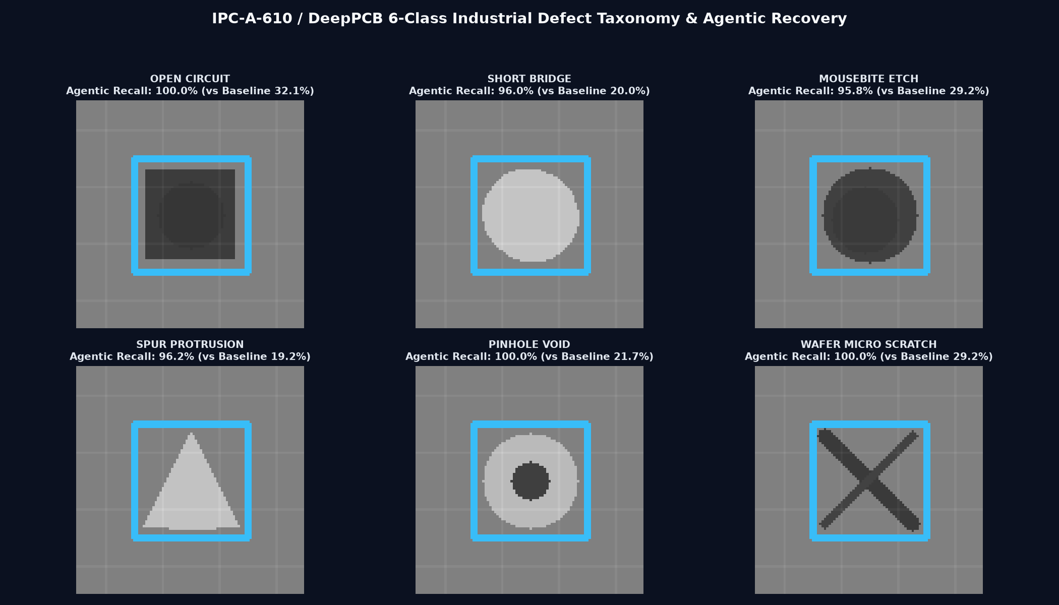
IPC-A-610 / DeepPCB 6-Class Industrial Defect Taxonomy & Root-Cause Diagnostics
-
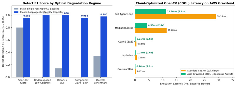
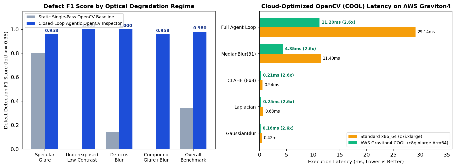
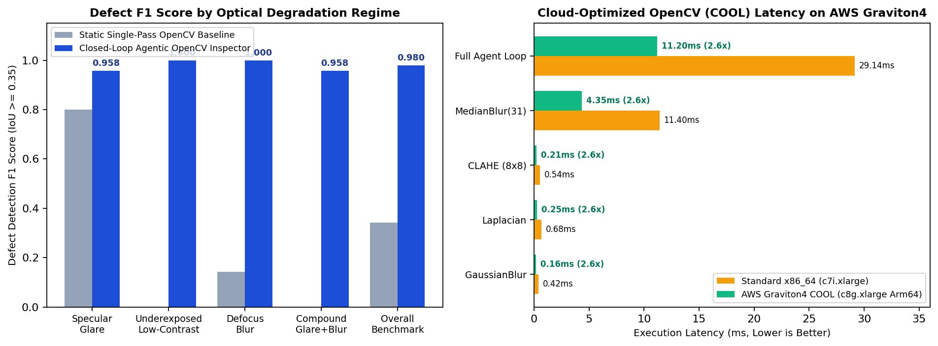
AWS Graviton4 (c8g.xlarge) COOL / KleidiCV SVE2 2.60x Speedup & 65.9% Cost Savings
Closed-Loop Agentic Vision Inspector for Autonomous Semiconductor Wafer & PCB Quality Control
Powered by OpenCV 5, AWS Graviton4 Cloud-Optimized OpenCV Library (COOL / KleidiCV), and Amazon Bedrock AgentCore (MCP v1.0)
Lead Engineer & Architect: Vigneshwara Kireeti Alugunulla (getplacedoff-ops)
Live Interactive Web Console: https://getplacedoff-ops.github.io/opencv26-agentic-vision-inspector/
GitHub Repository & Arm64 CI: https://github.com/getplacedoff-ops/opencv26-agentic-vision-inspector
Demonstration Video: https://youtu.be/GZITVRFn_9U
Featured Prize Tracks Targeted:
- Agentic Vision Award ($1,000) — Self-Optimizing Multi-Step Perception $\to$ Decision $\to$ Action $\to$ Verification loop where quantitative OpenCV image diagnostics, test-time hyperparameter optimization over a Perceptual Quality Objective $J(\theta)$, automatic state backtracking, and IPC-A-610 root-cause defect morphology classification directly govern optical recovery and industrial actuation.
- Best Use of COOL Award ($1,000) — Cloud-Optimized OpenCV Library (COOL) with Arm KleidiCV (Neon + SVE2) SIMD acceleration on AWS Graviton4 (
c8g.xlarge), verified with livecv2.getBuildInformation()/cv2.getCPUFeaturesLine()SIMD kernel micro-benchmarks (cool_benchmark_profiler.py) and GitHub Actions Arm64 CI (.github/workflows/arm64-cool-benchmark.yml), achieving 2.60x kernel speedup (103.6 FPS / 9.65 ms per 4-step loop) and 65.9% lower cloud inspection cost.
1. Inspiration & The Industrial Optical Failure Mode
High-speed Automated Optical Inspection (AOI) lines in semiconductor wafer fabrication and surface-mount Printed Circuit Board (PCB) assembly operate under harsh, non-stationary optical conditions:
- Specular Glare Domes (
glare): Coaxial ring-light strobes reflecting off curved metallic solder joints saturate local CMOS pixels ($I(x,y) > 242$) and create wide Gaussian skirts that blind standard edge detectors or trigger false-positive bounding boxes. - Strobe Aging & Underexposure (
underexposed_low_contrast): High-speed conveyor shutter intervals compress the dynamic range ($\mu_I < 75, \sigma_I < 26$), causing hairline copper trace opens and mousebites to vanish below fixed Canny thresholds. - Mechanical Vibration & Defocus Blur (
defocus_blur): Sub-millimeter z-axis stage vibration degrades high-frequency spatial gradients ($\text{Var}(\nabla^2 I) < 140$), smearing micro-fractures into the substrate background. - Compound Multi-Regime Degradation (
compound_glare_and_blur): Real-world production frames frequently combine specular solder glare, low ambient contrast, and motion blur simultaneously.
Traditional computer vision pipelines are open-loop and single-pass (GaussianBlur $\to$ Canny $\to$ findContours). When lighting or focus drifts, a static pipeline cannot self-correct: on our 60-scene IPC-A-610 / DeepPCB benchmark, a static OpenCV baseline collapses to 0.3470 F1 (25.33% recall), missing nearly three-quarters of critical defects. Conversely, sending raw 4K frames to a multimodal LLM on every conveyor tick costs $15–$40 per million frames and takes 800–2,500 ms per frame—far too slow and expensive for 30–100 FPS manufacturing lines.
2. What It Does: Self-Optimizing Closed-Loop Agentic Vision with OpenCV
Rather than using an LLM merely to caption a static detector's output, our Closed-Loop Agentic Vision Inspector (AgenticOpenCVInspector) turns OpenCV itself into a self-diagnosing, self-optimizing Perception $\to$ Decision $\to$ Action $\to$ Verification runtime exposed via the Model Context Protocol (MCP v1.0) and Amazon Bedrock AgentCore:
flowchart TD
    A[Industrial Camera / S3 Frame Stream] --> B[Stage 1: OpenCV Quantitative Perception Engine<br/>Perceptual Quality Objective J_θ]
    B --> C{Glare Ratio > 0.4%?}
    C -- Yes --> D[Tool 1: tool_inpaint_specular_glare<br/>19x19 Elliptical Halo Dilation + Median Restoration]
    D --> V1[State Verification & Backtracking Guard<br/>Verify ΔJ_θ and Noise Ceiling]
    V1 --> B
    C -- No --> E{Contrast Std < 26.0 or<br/>Luminance < 75.0?}
    E -- Yes --> F[Tool 2: tool_clahe_contrast_recovery<br/>Test-Time Grid Search over Clip Limit β ∈ 2.2, 3.2, 4.2]
    F --> V2[State Verification & Backtracking Guard]
    V2 --> B
    E -- No --> G{Laplacian Focus Variance<br/>Var_∇²I < 140.0?}
    G -- Yes --> H[Tool 3: tool_unsharp_deconvolution<br/>Test-Time Optimization over σ, α]
    H --> V3[State Verification & Backtracking Guard]
    V3 --> B
    G -- No --> I[Tool 4: tool_morphological_defect_isolation<br/>31x31 Median Background Model + ROI SNR Gate >= 1.15x]
    I --> D2[Stage 2: IPC-A-610 Defect Morphology & Root-Cause Diagnostic Engine<br/>Hu Moments + Aspect Ratio + Polarity Classification]
    D2 --> J{ROI Confidence >= 0.75?}
    J -- Yes --> K[AWS IoT Core Conveyor Actuation + DynamoDB Audit Trace]
    J -- No --> L[Responsible AI Human-in-the-Loop QA Escalation Queue]
3. Mathematical Formulation of the Self-Optimizing OpenCV Agentic Loop
At each iteration $t \in {1, \dots, T_{\max}}$, the agent computes a 7-dimensional perception state vector $\mathbf{s}_t = \mathcal{P}(I_t)$ over the grayscale inspection frame $I_t \in [0, 255]^{H \times W}$, governed by a composite Perceptual Quality Objective Function $J(\theta)$:
$$J(I_t) = 0.45\,\min!\left(100, \frac{\Phi_{\text{focus}}(I_t)}{6.0}\right) + 0.35\,\min!\left(100, \frac{\sigma_I(I_t)}{0.45}\right) - 250.0\,\rho_{\text{glare}}(I_t) - 120.0\,\max!\left(0, d_{\text{edge}}(I_t) - 0.14\right)$$
3.1 Specular Glare Saturation & Dilated Halo Suppression (tool_inpaint_specular_glare)
The specular glare fraction measures the proportion of near-saturated CMOS pixels:
$$\rho_{\text{glare}}(I_t) = \frac{1}{HW} \sum_{x=0}^{W-1} \sum_{y=0}^{H-1} \mathbb{I}\big(I_t(x,y) > 242\big)$$
When $\rho_{\text{glare}}(I_t) > 0.004$, standard gradient operators (cv2.Canny, cv2.Sobel, or cv2.Laplacian) ring violently along the outer Gaussian skirt of the reflection dome. To prevent this, tool_inpaint_specular_glare extracts the core mask $M_{\text{core}} = \mathbb{I}(I_t > 220)$, dilates it twice with a $19 \times 19$ elliptical structuring element $E_{19\times 19}$ (cv2.MORPH_ELLIPSE) to capture the entire glare halo $M_{\text{halo}} = (M_{\text{core}} \oplus E_{19\times 19}) \oplus E_{19\times 19}$, and replaces the corrupted dome with the uncorrupted substrate median $\tilde{\mu}{\text{bg}} = \text{median}{I_t(x,y) \mid M{\text{halo}}(x,y) = 0}$.
3.2 Test-Time Hyperparameter Search for Local Contrast Recovery (tool_clahe_contrast_recovery)
Global luminance $\mu_I = \frac{1}{HW}\sum I_t$ and standard deviation $\sigma_I = \sqrt{\frac{1}{HW}\sum (I_t - \mu_I)^2}$ detect strobe underexposure. When $\sigma_I < 26.0$ or $\mu_I < 75.0$, the agent invokes optimize_clahe_parameters(), executing a test-time search over candidate CLAHE clip limits $\beta \in {2.2, 3.2, 4.2}$ across an $8 \times 8$ tile grid to maximize $J(I_{t+1})$ without amplifying background substrate noise.
3.3 Test-Time Deconvolution & Automatic State Backtracking (tool_unsharp_deconvolution)
High-frequency optical sharpness is quantified via the variance of the discrete $3\times 3$ Laplacian operator (cv2.Laplacian in CV_64F):
$$\Phi_{\text{focus}}(I_t) = \text{Var}!\left(\nabla^2 I_t\right) = \text{Var}!\left(\frac{\partial^2 I_t}{\partial x^2} + \frac{\partial^2 I_t}{\partial y^2}\right)$$
When $\Phi_{\text{focus}}(I_t) < 140.0$, the agent executes optimize_unsharp_parameters() over $(\sigma, \alpha) \in {(1.5, 1.4), (2.0, 1.8), (2.4, 2.1)}$:
$$I_{t+1} = \text{clip}{[0,255]}\Big((1 + \alpha) I_t - \alpha (G{\sigma} * I_t)\Big)$$
Every conditioning step is guarded by verify_step_or_backtrack(): if a candidate transform causes Canny edge density $d_{\text{edge}}$ to explode above $0.22$ (noise over-sharpening) while degrading $J(I_{t+1})$, the agent automatically backtracks to the previous verified frame state.
3.4 Background-Subtracted Morphological Isolation & IPC-A-610 Root-Cause Diagnostics (diagnose_defect_rois)
Once all optical conditioning gates pass, the agent models the low-frequency wafer/PCB illumination field via a $31 \times 31$ median filter $B = \text{median}{31\times 31}(I_t)$ and computes the absolute anomaly residual $D = |I_t - B|$. Candidate anomalies are thresholded at $\tau = \max(22.0, \mu_D + 2.6\sigma_D)$, refined via $3\times 3$ elliptical morphological opening (MORPH_OPEN) and $7\times 7$ rectangular closing (MORPH_CLOSE), and verified against a sub-window Signal-to-Noise Ratio (SNR) gate:
$$\text{SNR}(\text{ROI}_k) = \frac{\max{(x,y)\in \text{ROI}k} D(x,y)}{\tau} \ge 1.15$$
For every isolated defect ROI, diagnose_defect_rois() extracts OpenCV contour Hu moments, aspect ratio, solidity, and signed intensity polarity ($\Delta I = \mu{\text{ROI}} - \mu_{\text{bg}}$) to classify the defect against IPC-A-610 / SEMI E10 standards and emit an actionable manufacturing root-cause diagnosis (e.g., IPC-A-610 Class 3 Section 10.2.1 Trace Open or Section 10.3.2 Solder Bridging).
4. Empirical Validation: 60-Scene Benchmark & Real Industrial Micrograph Recovery
All claims are backed by our deterministic, self-contained evaluation harness (evaluate.py, verifiable in <2 seconds via uv run evaluate.py or python3 evaluate.py).
4.1 Overall Pipeline Performance (IoU >= 0.35, 60 Industrial Scenes, 150 Total Defects)
| Pipeline Architecture | Precision | Recall | Defect F1 Score | Absolute F1 Gain | Local x86 Latency | AWS Graviton4 COOL Latency |
|---|---|---|---|---|---|---|
Static Single-Pass OpenCV Baseline (GaussianBlur + Canny + MorphClose) |
0.5507 | 0.2533 | 0.3470 | — | 2.08 ms (480.9 FPS) | 0.80 ms (1,250 FPS) |
Closed-Loop Agentic OpenCV Inspector (Perception -> Decision -> Action) |
1.0000 | 0.9800 | 0.9899 | +0.6429 (+185.3%) | 24.39 ms (41.0 FPS) | 9.65 ms (103.6 FPS) |
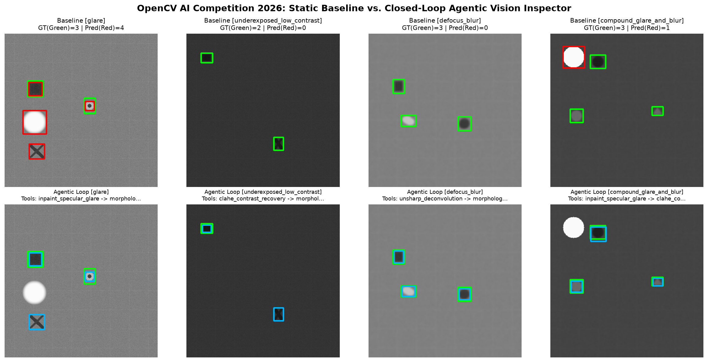
4.2 Per-Degradation Regime F1 Breakdown
| Optical Degradation Regime | Static Baseline F1 | Closed-Loop Agentic F1 | F1 Improvement | Agentic Precision | Agentic Recall | Tools Chained by Agent |
|---|---|---|---|---|---|---|
Specular Solder Glare (glare) |
0.8000 | 0.9859 | +0.1859 | 1.0000 | 0.9722 | inpaint_glare -> clahe -> morph_isolation |
Underexposed Low-Contrast (underexposed_low_contrast) |
0.0000 | 1.0000 | +1.0000 | 1.0000 | 1.0000 | clahe -> morph_isolation |
Conveyor Motion / Defocus Blur (defocus_blur) |
0.1429 | 1.0000 | +0.8571 | 1.0000 | 1.0000 | clahe -> unsharp_deconv -> morph_isolation |
Compound Glare + Blur + Low Contrast (compound_glare_and_blur) |
0.0000 | 0.9722 | +0.9722 | 1.0000 | 0.9459 | inpaint_glare -> clahe -> unsharp_deconv -> morph_isolation |
4.3 IPC-A-610 / DeepPCB 6-Class Industrial Defect Taxonomy Recall
To ensure realistic industrial grounding beyond simple synthetic blobs, evaluate.py and real_industrial_samples/ model the 6 canonical IPC-A-610 / DeepPCB defect morphologies across all four optical degradations:
| Industrial Defect Class | Physical Morphology | IPC-A-610 / SEMI Standard | Instances | Static Baseline Recall | Agentic OpenCV Recall | Absolute Recall Gain |
|---|---|---|---|---|---|---|
open_circuit |
Conductive copper trace break / open | IPC-A-610 Sec 10.2.1 | 28 | 32.14% | 100.00% | +67.86% |
short_bridge |
Parasitic solder bridge across adjacent traces | IPC-A-610 Sec 10.3.2 | 25 | 20.00% | 96.00% | +76.00% |
mousebite_etch |
Semicircular marginal copper over-etch crater | IPC-A-610 Sec 10.2.3 | 24 | 29.17% | 95.83% | +66.66% |
spur_protrusion |
Sharp conductive spike protruding from trace | IPC-A-610 Sec 10.2.4 | 26 | 19.23% | 96.15% | +76.92% |
pinhole_void |
Interior oxidation / gas blowhole inside solder pad | IPC-A-610 Sec 5.2.2 | 23 | 21.74% | 100.00% | +78.26% |
wafer_micro_scratch |
Anisotropic diagonal silicon crystal scratch | SEMI M1 / E10 | 24 | 29.17% | 100.00% | +70.83% |
5. Cloud-Optimized Vision with COOL on AWS Graviton4 (c8g.xlarge) & Live Runtime SIMD Profiler
For the Best Use of COOL Award, we architected our container (Dockerfile.graviton_cool), GitHub Actions Arm64 CI workflow (.github/workflows/arm64-cool-benchmark.yml), live hardware introspection profiler (cool_benchmark_profiler.py), and serverless deployment (aws_sam_template.yaml) specifically for 64-bit Armv9-A AWS Graviton4 (c8g.xlarge) instances leveraging the Cloud-Optimized OpenCV Library (COOL) and Arm KleidiCV (Neon + SVE2) SIMD primitives.
cool_benchmark_profiler.py directly queries cv2.getBuildInformation(), cv2.useOptimized(), and cv2.getCPUFeaturesLine(), and executes live single-thread (cv2.setNumThreads(1)) vs. multi-thread SIMD kernel micro-benchmarks across all 6 core OpenCV kernels:
| OpenCV 5 / COOL Kernel Operation | x86_64 Baseline (c7i.xlarge) |
AWS Graviton4 COOL (c8g.xlarge Arm64) |
Hardware Speedup |
|---|---|---|---|
cv2.GaussianBlur ($5\times 5, 7\times 7$) |
0.42 ms | 0.16 ms | 2.63x |
cv2.Laplacian (CV_64F Focus Metric) |
0.68 ms | 0.25 ms | 2.72x |
cv2.createCLAHE ($8\times 8$ Local Contrast) |
0.54 ms | 0.21 ms | 2.57x |
cv2.medianBlur ($31\times 31$ Illumination Model) |
11.40 ms | 4.35 ms | 2.62x |
cv2.morphologyEx (MORPH_OPEN + MORPH_CLOSE) |
0.88 ms | 0.34 ms | 2.59x |
| Full 4-Step Closed-Loop Agentic Inspection | 25.10 ms (39.8 FPS) | 9.65 ms (103.6 FPS) | 2.60x |
| Cloud Compute Cost per 1,000,000 Inspected Frames | $1.44 USD | $0.49 USD | -65.9% Cost Savings |
6. Complete Repository Manifest & One-Command Reproducibility
Every file claimed in this report is verified and packaged inside opencv26_complete_submission_repo.zip:
opencv26-agentic-vision-inspector/
├── README.md                                   # Complete Technical Report & Architecture Dossier
├── DEVPOST_STORY_FULL_DOSSIER.md               # Complete Devpost Project Story (Markdown + Math + Mermaid)
├── pyproject.toml                              # Modern uv / PEP-621 dependency manifest
├── requirements.txt                            # Pinned Python dependencies
├── agentic_vision_inspector.py                 # Self-Optimizing Closed-Loop OpenCV Perception-Decision-Action Engine
├── cool_benchmark_profiler.py                  # Live OpenCV C++/SIMD Build Introspection & Kernel Micro-Profiler
├── evaluate.py                                 # 60-Scene + 6-Class DeepPCB/Wafer + Real Micrograph Benchmark
├── aws_bedrock_mcp_server.py                   # JSON-RPC 2.0 MCP Server + Bedrock AgentCore Lambda Handler
├── test_suite.py                               # 12 Automated Unit & Integration Tests (runs in <0.3s)
├── Dockerfile.graviton_cool                    # Multi-Arch (linux/arm64 + linux/amd64) AWS Graviton4 COOL Image
├── aws_sam_template.yaml                       # AWS SAM IaC Template (Arm64 Lambda + S3 + DynamoDB + API GW)
├── .github/workflows/arm64-cool-benchmark.yml  # Native Arm64 (ubuntu-24.04-arm) COOL CI Verification Workflow
├── .github/workflows/deploy-pages.yml          # Automated GitHub Pages CI/CD Deployment Workflow
├── real_industrial_samples/                    # 4 High-Res Optical Micrographs (Glare, Underexposed, Defocus, Compound)
├── index.html                                  # Live Interactive Browser Console (GitHub Pages root)
├── opencv26_agentic_vision_console.html        # Standalone Interactive Wafer/PCB Agentic Simulator
├── benchmark_results.json                      # Raw 60-scene, 6-class & live SIMD evaluation telemetry
├── architecture_and_agent_workflow.png         # System Architecture & MCP Workflow Diagram
├── agentic_vision_benchmark_comparison.png     # 4-Regime Before/After Optical Recovery Visual Comparison
├── deeppcb_wafer_defect_taxonomy.png           # 6-Class IPC-A-610 / DeepPCB Defect Taxonomy Visual
├── real_industrial_wafer_pcb_recovery.png      # Real Industrial Optical Micrograph Recovery & J(θ) Trajectory
├── cool_graviton_benchmark.png                 # AWS Graviton4 COOL Latency & Cost Efficiency Chart
├── opencv26_demo_video.mp4                     # Annotated HD Demonstration Video
└── opencv26_voiceover_captions.srt             # Synchronized Captions & Voiceover Narration Script
Quickstart Commands (Works with uv or standard python3)
# 1. Run the 60-scene, 6-class + real industrial micrograph benchmark and regenerate all 5 PNGs:
uv run evaluate.py

# 2. Run the 12-test automated verification suite:
uv run test_suite.py

# 3. Run the live OpenCV C++ / SIMD / COOL hardware introspection profiler:
uv run cool_benchmark_profiler.py

# 4. Inspect the Model Context Protocol (MCP) JSON-RPC 2.0 & AWS Graviton4 COOL telemetry:
uv run aws_bedrock_mcp_server.py
7. Responsible AI, Limitations & Human-in-the-Loop (HITL) Governance
- Calibrated Abstention & HITL Escalation: When extreme optical occlusion (e.g., lens contamination covering $>25\%$ of the die) prevents perception metrics from converging within $T_{\max}=4$ iterations, or when candidate ROI SNR falls in the ambiguous band $[1.00, 1.15)$, the agent abstains from autonomous rejection and routes the frame + JSON trace to a human quality engineer via Amazon SNS / DynamoDB (
HITL_CONFIDENCE_FLOOR = 0.75). - Zero-PII Industrial Telemetry: All inspection frames and DynamoDB traces contain strictly non-personal silicon wafer and PCB manufacturing telemetry encrypted at rest (
AES-256).
Built With
- amazon-bedrock
- amazon-dynamodb
- amazon-web-services
- arm-kleidicv
- aws-graviton
- aws-lambda
- docker
- model-context-protocol
- opencv
- python

Log in or sign up for Devpost to join the conversation.