-
-
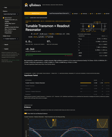
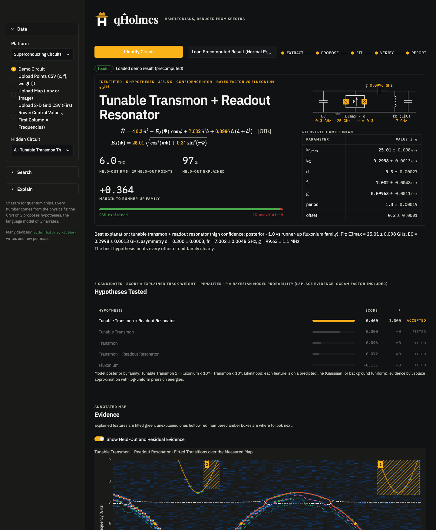
UI
-
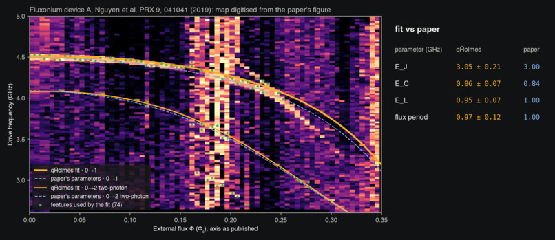
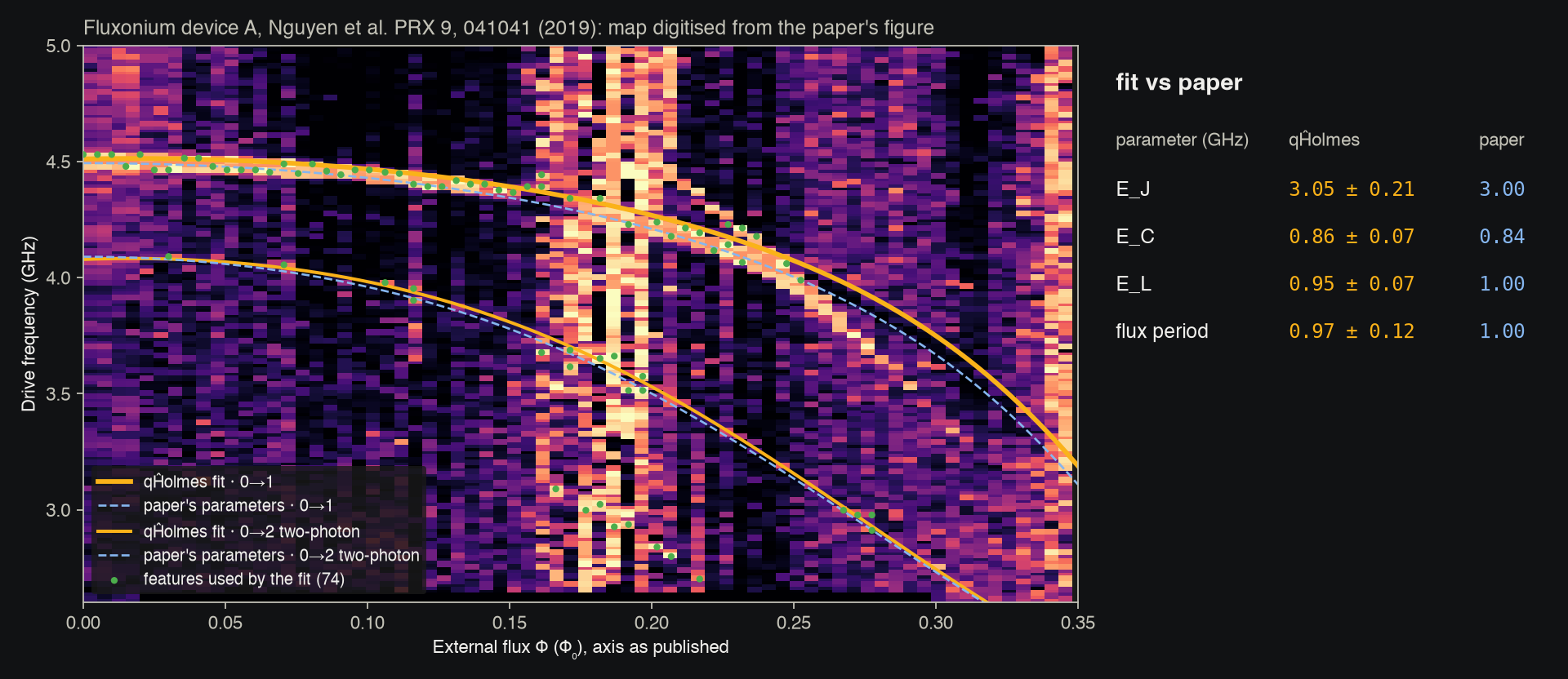
Published fluxonium map (Nguyen et al., PRX 2019), no tuning: qĤolmes's fit (amber) over the paper's own parameters (dashed)
Inspiration
When in a circuit QED lab, every new chip starts the same way for me: a two-tone spectroscopy map comes off the fridge, I stare at a screen full of lines, and I start guessing which circuit made them and what its energies are. It is slow, it is easy to get wrong, and if I get it wrong every calibration I do afterwards inherits the mistake. I have lost whole days to this, and when I talked to people who work with NV centres, quantum dots, trapped ions and Rydberg atoms, they described the same ritual with different lines. That was the inspiration: the map already contains the Hamiltonian, so I wanted a tool that reads it out the way a physicist would, by trying real models against the data and being honest about what does not fit.
What it does
Upload a spectroscopy map (image, NPZ, HDF5 or a CSV of features) from one of five platforms and qĤolmes
- extracts the spectral features and separates flux-dependent lines from pumps and spurs,
- proposes device families (a CNN trained on 190,000 synthetic maps only proposes; it never decides),
- fits every hypothesis with the actual Hamiltonian (transmon, flux-tunable transmon, fluxonium with and without a readout resonator, NV ensemble, double-dot charge qubit, trapped-ion sidebands, Rydberg Stark map) using a robust global search,
- verifies on held-out flux columns, reports Jacobian uncertainties calibrated by coverage runs, and samples the posterior on demand,
- compares the models two ways: a feature-level score and a Bayesian model posterior from Laplace evidences, shown as a Bayes factor,
- lists what it cannot explain and interprets it (a tone the qubit crosses without splitting is a pump, not a resonator),
- designs the next measurement by Fisher information (expected information gain in bits per sweep) and runs a closed-loop autopilot on a digital twin,
- derives the spec sheet a lab needs (sweet spots, anharmonicity, dispersive shift by exact diagonalisation, flux-noise Tφ),
- answers questions in plain language through Ask qĤolmes, where Claude calls the physics engine as tools so every number is traceable,
- exports the report, the fitted curves, the annotated map and a scqubits snippet; the same engine is a CLI and a REST API.
The Hamiltonian it recovers is typeset with the fitted numbers in place, for example
$$\hat H = 4 E_C \hat n^2 - E_J(\Phi)\cos\hat\varphi + f_r \hat a^\dagger \hat a + g\,\hat n(\hat a + \hat a^\dagger),\qquad E_J(\Phi) = E_{J,\max}\sqrt{\cos^2(\pi\Phi) + d^2 \sin^2(\pi\Phi)}.$$
How we built it
Python, NumPy and SciPy for batched Hamiltonians (charge basis for transmons, oscillator basis for fluxonium, resonator dressing by exact diagonalisation with overlap labelling), checked against scqubits to 1 kHz in the test suite. Feature extraction is a robust per-column peak finder with sub-pixel refinement and slope-aware track linking. Fitting is an annealed differential evolution over a Geman–McClure nearest-line loss, followed by a two-stage soft-L1 polish, multi-start, and explicit alternatives for the label ambiguities we discovered (two-photon versus thermal line, first- versus second-order sideband, a hyperbola versus its two-photon copy). Hold-out verification, Laplace covariances, Metropolis posterior sampling and Fisher-information design sit on top of the same objective. A small CNN proposer was trained on synthetic maps generated on a 32-core machine. The interface is Streamlit with Plotly and KaTeX; Claude Opus 5.5 writes the two-sentence summary (structured output) and powers the tool-using assistant. FastAPI exposes the engine, a Dockerfile packages it, and GitHub Actions runs the physics, extraction and API suites on every push.
Challenges we ran into
Spurs. A pump tone is a perfectly straight line that any flexible model loves to explain; the fix was to score features, not pixels, to remove flat lines before flux-dependent fits, and to accept a resonator only when it explains flux-dependent evidence. Degeneracies: EJ and EC trade off along constant f01, so the report says so and asks for the two-photon line. Label ambiguities cost a factor of two silently until blind tables at scale (200 random devices per platform on a 20-core machine) exposed them; teaching the fitter to try the other reading raised trapped ions from 74 % to 86 % and quantum dots from 58 % to 78 % of devices with every parameter within 5 %. Heavy fluxoniums whose tuning sits outside the measured band still get read as fixed transmons, and we say so.
Accomplishments that we're proud of
A published fluxonium map (Nguyen et al., PRX 2019), digitised from the paper's figure with no tuning, comes back as EJ = 3.05 ± 0.21 GHz, EC = 0.86 ± 0.07 GHz, EL = 0.95 ± 0.07 GHz against the paper's 3.0 / 0.84 / 1.0 (the error bars reflect the figure's 12.5 MHz pixels), with the flux period recovered as one flux quantum. Family identification is 200/200 on ions, NV centres, dots and Rydberg atoms in blind tests, and the fitter knows when it is unreliable: the maps it gets wrong carry a low score and a warning. The Bayes factor and the Fisher design are computed, not narrated.
What we learned
That a physics fit with honest scoring beats a learned regressor when the data contain things the model does not describe, and that the most useful output of a fitter is the list of what it could not fit together with the measurement that would settle it. Also that blind tables are the fastest way to find the failure mode you did not know you had.
What's next for qĤolmes
Real data, from real labs. One published fluxonium map is a start, not a validation set: the next step is collecting raw spectroscopy maps from groups working on superconducting circuits, NV centres, quantum dots, trapped ions and Rydberg atoms, with their own fits as ground truth, and tuning the extractor and the priors against that instead of against our synthetic generator. We want each subfield to tell us what its maps really look like (the pumps, the drifts, the line shapes) and what it needs read off them. From there: connect the "look here" suggestion to an instrument driver so the autopilot runs on the real fridge; add 0–π and coupled-transmon families; ridge-following extraction for very noisy maps; and a defect census that catches small avoided crossings along the qubit line.

Log in or sign up for Devpost to join the conversation.