Chevron Hot Dog Prediction

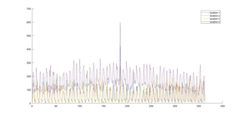
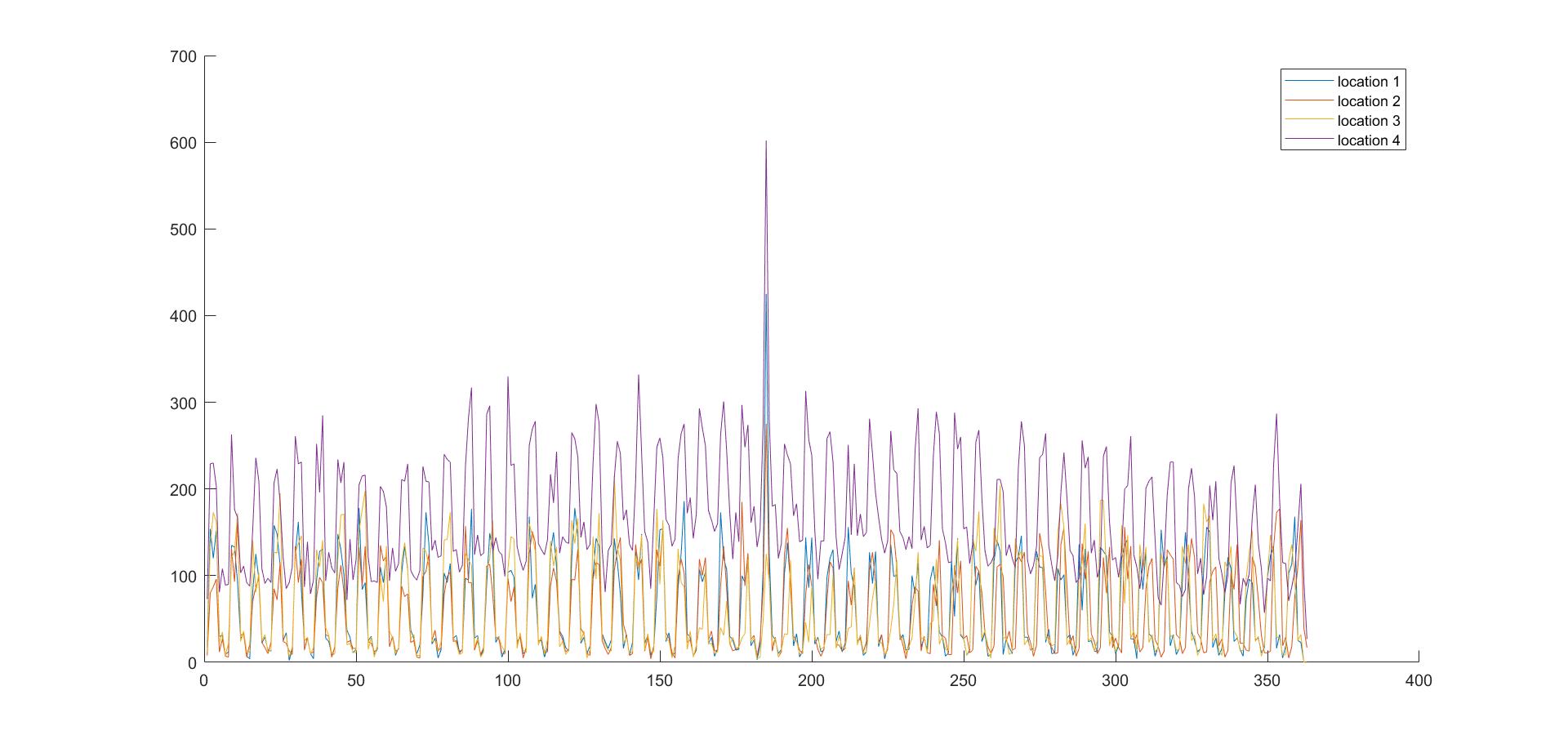
Figure 1: Cumulative daily demand for each location
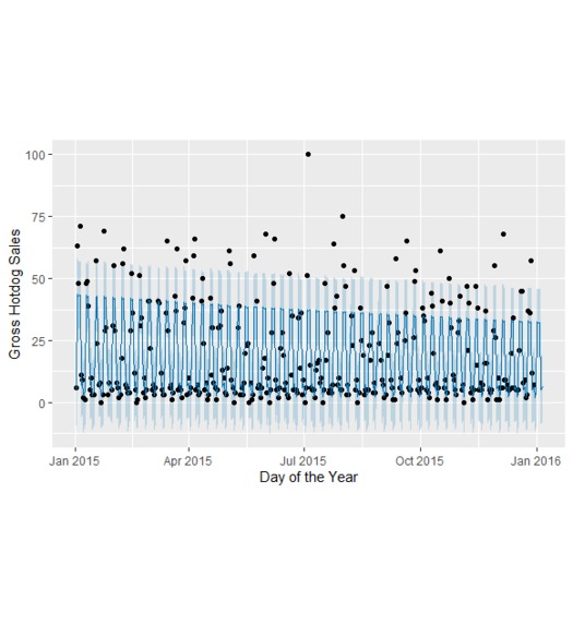
Figure 2: Store 1000, Time bucket 3 - fit model
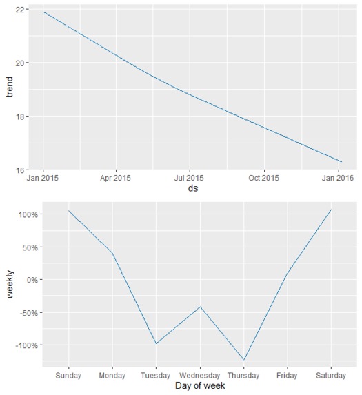
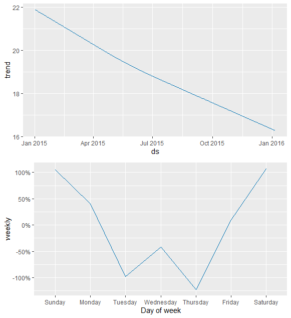
Figure 3: Store 1000, Time Bucket 3 - components

Methodology

Since we determined that each store was located in a different city and had different characteristics, with regards to the presence of a car wash, whether alcohol was sold, and differing payment methods, we found it useful to split our analysis into a store-by-store basis. Therefore, we created the same model, but applied it separately to different stores. We decided to not look for correlation between these characteristics and the demand, because the sample size of four stores is not sufficient to draw any conclusions of this sort.

We further split our analysis of each store into each three-hour bucket. In other words, our analysis for a single store consisted of four different applications of the model, with a separate analysis for each three-hour bucket. For example, we generated separate predictions for store_1000 during hour bucket 1, store_1000 during hour bucket 2, store_1000 during hour bucket 3, and store_1000 during hour bucket 4. We repeated this process for all four stores.

Our model employed the use of the R package Prophet. Prophet requires a single column of date/time data, so we first had to transform the integers for days of the year and times of the day into a single format for use in R. We arbitrarily chose Jan. 1, 2015 as our starting date for our 363 days of data because the data peaked 2-3 days a week, which we assumed was Friday-Sunday and found a recent year that aligned with our assumption that three-day peaks in the data corresponded to Friday, Saturday, and Sunday. Our time assigned to each bucket was the starting time of the bucket (i.e. 8am for bucket 1). In the implementation, we used Prophet to fit a curve to each data set relying on a weekly seasonality and a multiplicative seasonality effect (as opposed to the default additive effect). The seasonality allowed our curve to account for days of the week and cycle appropriately, while the multiplicative allowed the curve to adjust to the changing range of the data over time. After fitting the model to our data, we used the curve to extrapolate into the future, specifically forecasting days 364 & 365. The data will be rounded up to the next integer number of hot dogs sold to account for the sale of full hot dogs.

We decided to not exclude the outlier, day 185 from the database because the influence of this one day on the overall model is minimal.

In addition to the model, we visualized the training data by plotting daily demand of each location on one graph, as presented on Figure 1 (See media above or PDF on GitHub for figures).

Findings

From our model we saw several overall tendencies:

cyclical nature of the demand for each bucket/day, with a period of 7 days
3 consecutive days out of 7 corresponded to a peak, most likely the weekends. We assumed that these three days corresponded to Friday, Saturday, and Sunday
location 4 demonstrated higher mean and baseline, while other locations’ demand was rather close together, as well as bigger seasonality
for each location, day 185 (likely July 4th) produced an unusual spike, an outlier

We produced a model predicting demand at each location at each time bucket 7 days into the future as well as at missing values. Note that based on our weekday assumption above, we conjectured that the data came from a year that started on a Thursday, the most recent of which was 2015. An example plot of the resulting curve fit (for store 1000, time bucket 3) is shown below on Figure 2 (See media above or PDF on GitHub for figures). Different graphs and curve fits were generated for each store during each hour block. Additionally, the overall weekly and monthly components of our model are shown in Figure 3. Our model does have a drawback in that it tends to more readily predict low values of sold hot dogs more easily than high values, so future work in Prophet will adjust parameters such that the curve more accurately captures higher numbers.