CASCADE Compound Risk Intelligence for Southern California
Inspiration When the Palisades Fire tore through LA in January 2025, something less visible happened after the flames went out. Ash runoff entered the ocean, deepening hypoxic zones already stressed by a warming Pacific. The grid, weakened by heat waves and wildfire shutoffs, inched toward cascading failure. Each of these domains has a dedicated warning system. USGS watches faults. NOAA and CalCOFI watch the ocean. Utilities watch the grid. But no one watches them together, and the disasters that actually hurt us are rarely single-domain events — they are cascades. CASCADE is our answer to a simple question: what if a system could watch all four domains at once and explain, in plain English, what happens when they align?
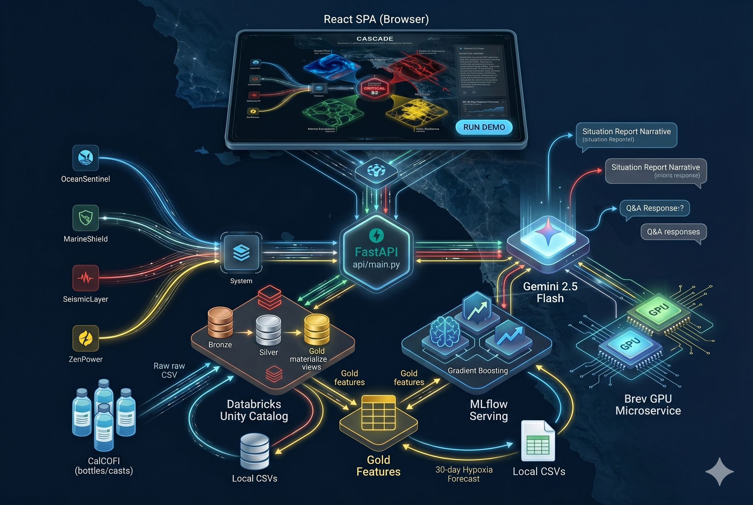
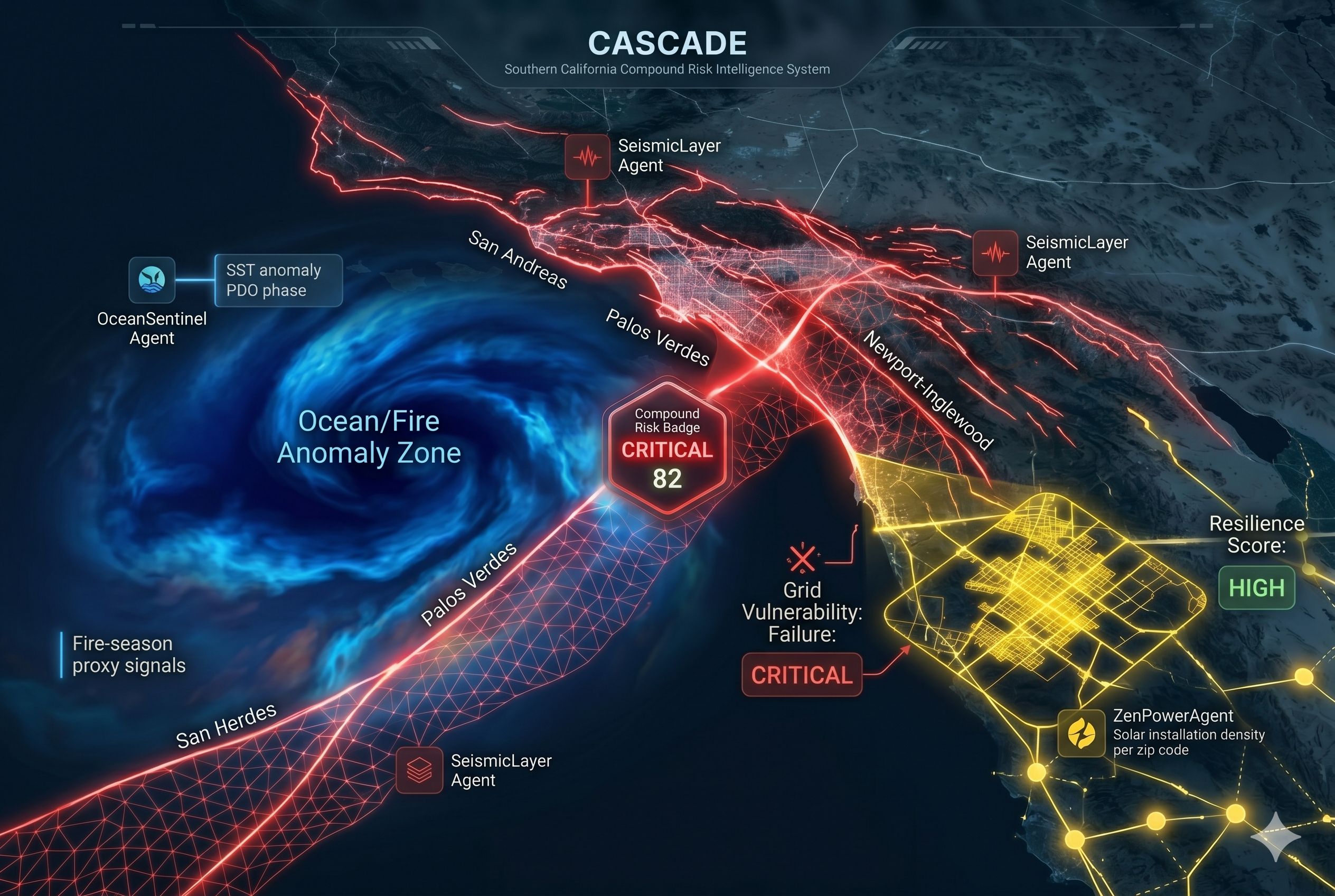
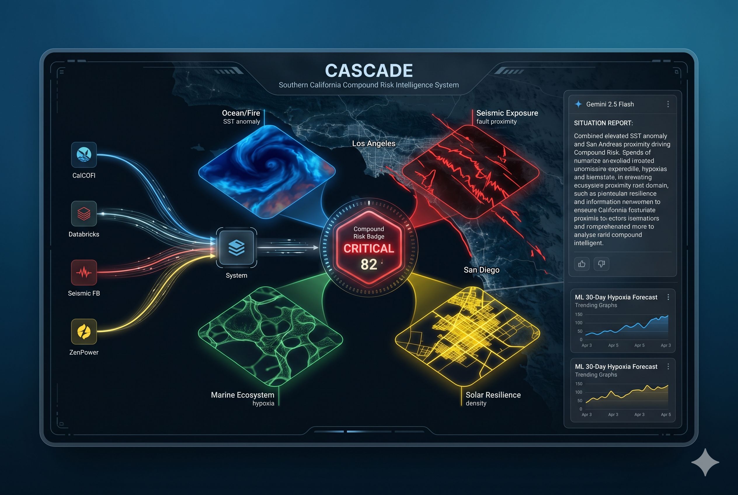
What It Does CASCADE fuses four independent hazard domains into a single compound risk score for Southern California, updated in real time: DomainSignalOceanSST anomaly, PDO phase, La Niña indicators, fire season riskMarineDissolved oxygen, hypoxia risk, ML-forecasted next-month conditionsSeismicFault proximity, compound zone overlap, GPU-accelerated geometryGridSolar install density, grid vulnerability, resilience scoring The score is surfaced through an interactive Leaflet map, an ML forecast card for next-month marine conditions, a Gemini-generated situation report, a chat interface with memory, and a historical replay mode that reconstructs the compound risk state for any past date. The scoring function is a weighted fusion of the four agent alerts: compound_score=0.30⋅ocean+0.25⋅marine+0.25⋅seismic+0.20⋅grid\text{compound_score} = 0.30 \cdot \text{ocean} + 0.25 \cdot \text{marine} + 0.25 \cdot \text{seismic} + 0.20 \cdot \text{grid}compound_score=0.30⋅ocean+0.25⋅marine+0.25⋅seismic+0.20⋅grid
How We Built It Data — Databricks Medallion Pipeline We built on CalCOFI, one of the longest-running ocean monitoring programs on Earth: 650,790 bottle measurements across 70+ years of Southern California coastal science (1949–2021). Raw CSVs landed in Unity Catalog and flowed through a three-stage Lakeflow Declarative Pipeline:
Bronze — raw columns, no transformations, preserved for lineage. Silver — cleaned, joined (bottle LEFT JOIN cast ON Cst_Cnt), type-cast, filtered by quality gates. 650,790 rows. Gold — aggregated by year_month into 467 monthly regional features. Each row represents one month of Southern California ocean state averaged across all sampled stations.
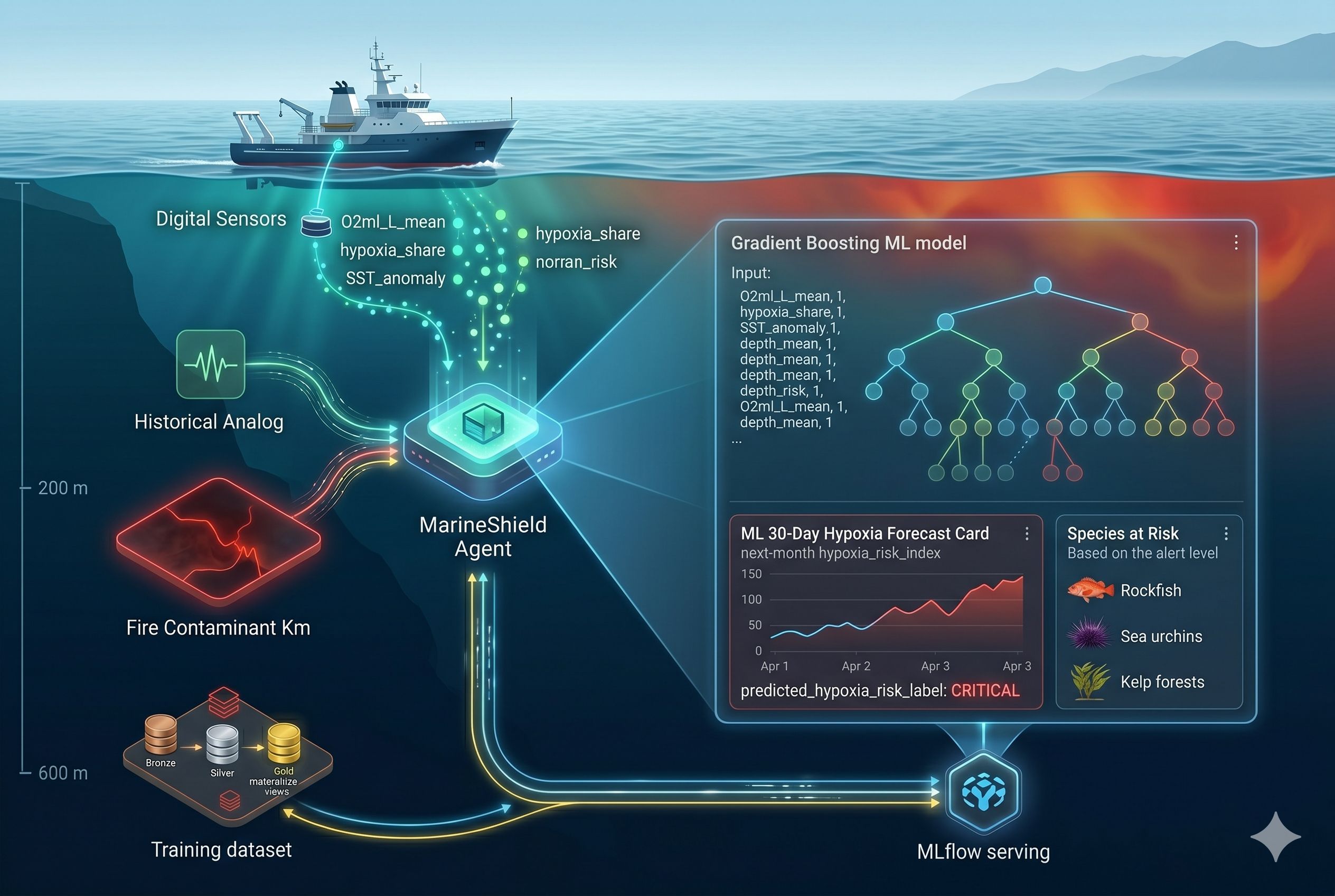
Core derived columns computed in gold: hypoxia_share=1N∑i=1N1 [O2,i<2.0 mL/L]\text{hypoxia_share} = \frac{1}{N} \sum_{i=1}^{N} \mathbb{1}!\left[O_{2,i} < 2.0 \text{ mL/L}\right]hypoxia_share=N1i=1∑N1[O2,i<2.0 mL/L] sst_anomaly=surface_temp_mean−climatologymonth\text{sst_anomaly} = \text{surface_temp_mean} - \text{climatology}{\text{month}}sst_anomaly=surface_temp_mean−climatologymonth Machine Learning — GradientBoosting with TimeSeriesSplit A LEAD shift on the 467 monthly rows produced next-month targets and 466 training rows across 12 features. Two GradientBoostingRegressor models were trained — one for target_next_hypoxia_risk_index, one for target_next_O2ml_L_mean — registered in the MLflow Model Registry under @champion aliases and deployed as Databricks Model Serving endpoints. The critical design choice was TimeSeriesSplit cross-validation: Foldk:train=[0, tk),validate=[tk, tk+1)\text{Fold}_k: \quad \text{train} = [0, \, t_k), \qquad \text{validate} = [t_k, \, t{k+1})Foldk:train=[0,tk),validate=[tk,tk+1) Standard k-fold would randomly shuffle rows, training on November 2005 while validating on March 2002 and leaking the future into the past. TimeSeriesSplit guarantees training is always chronologically before validation, mirroring real deployment. Multi-Agent Orchestration Four agents run in parallel on every /api/status call:
OceanSentinel — derives La Niña and PDO signals from SST and salinity; estimates fire-season risk. MarineShield — reads hypoxia and dissolved oxygen; calls the MLflow endpoint for a 30-day forecast. SeismicLayer — HTTP-calls a Brev-hosted GPU microservice for fault-proximity geometry. ZenPowerAgent — reads solar install density and grid vulnerability per zip code.
The orchestrator weights their outputs, computes the compound score, and passes the full state to Gemini 2.5 Flash for narrative generation. LLM Layer Gemini 2.5 Flash was chosen for its latency profile — Pro and Ultra are too slow for a dashboard that refreshes every 30 seconds. The LLM handles situation report generation and chat with conversational memory, where /api/ask passes prior turns in the prompt to support follow-up questions. Frontend frontend/index.html is a single file — React 18 via CDN, Babel standalone for in-browser JSX, Tailwind for styling, Leaflet for the map. No npm install, no bundler, no build step. Graceful Fallback Every external dependency has a fallback tier. Databricks down falls back to local CalCOFI CSVs. A failed serving endpoint falls back to a local MLflow artifact, then to heuristic-only output. Gemini down falls back to canned narratives. Brev down falls back to local seismic heuristics. The demo never crashes.
Challenges We Ran Into
Small-data ML on 466 rows We had 650,790 raw measurements but trained on only 466 rows. The aggregation was intentional — each row represents one month of regional state, which is the correct granularity for monthly forecasting — but small-data ML is genuinely harder to defend. We leaned on TimeSeriesSplit discipline, regularized hyperparameters (max_depth=4\text{max_depth}=4 max_depth=4, learning_rate=0.05\text{learning_rate}=0.05 learning_rate=0.05, subsample=0.8\text{subsample}=0.8 subsample=0.8), and honest evaluation to produce a model we trusted.
CalCOFI ends in May 2021 We wanted to replay the Palisades Fire in January 2025, but CalCOFI stops in mid-2021. Our solution was two-layered. For representative demo dates (2024-11-01 and 2025-01-07), we hardcode realistic agent values and always generate a fresh Gemini narrative, clearly flagged as representative_scenario in the UI. For arbitrary post-2021 queries, we use cosine similarity in feature space to find the closest historical analog month: similarity(x,y)=x⋅y∥x∥ ∥y∥\text{similarity}(\mathbf{x}, \mathbf{y}) = \frac{\mathbf{x} \cdot \mathbf{y}}{|\mathbf{x}| \, |\mathbf{y}|}similarity(x,y)=∥x∥∥y∥x⋅y Every post-2021 date returns a coherent, physically plausible state grounded in real historical oceanography rather than fabricated numbers.
Python 3.12/3.13 MLflow artifact compatibility Loading a scikit-learn model trained in one Python version from a local artifact in another produced compatibility warnings and occasional silent prediction drift. We resolved this by preferring Databricks Model Serving over local artifact loading — the endpoint runs its own containerized Python environment that matches training.
The feature vector ordering trap Our models train on 12 features in a specific order. At inference, reordering the list produces silently wrong predictions — no error, just bad numbers. We hardcoded a single FEATURES constant and routed every inference call through it, eliminating an entire class of silent bugs.
What We Learned The medallion architecture earns its complexity. Bronze/silver/gold felt like over-engineering on day one. By day two we had re-run transformations multiple times against preserved bronze data, each time catching a silver-layer bug that would have required a full re-upload otherwise. Keeping raw data immutable is a superpower. Time-series ML is a different discipline. Random k-fold looks innocuous until you realize it is quietly letting the model cheat. TimeSeriesSplit and the LEAD/LAG window functions that create proper next-month targets are not optional for temporal forecasting. LLMs belong in the narrative layer, not the decision layer. Our compound score is weighted, not learned — coefficients we can justify to a stakeholder. Gemini writes the briefing but does not compute the score. This separation keeps the system interpretable. Emergency managers need to trust the number; the LLM just makes it readable. Graceful degradation is the best demo strategy. Every external dependency fails eventually. Designing for failure from the start meant the demo survived everything, including Wi-Fi outages mid-presentation. Fusion beats monitoring. The disasters that hurt us are not individual events, they are cascades. Any system that monitors a single domain, no matter how well, misses the real story. Compound risk intelligence is a missing category in the monitoring stack, and we think it is the next one.
What's Next for CASCADE
Live data integration with USGS earthquake catalogs, CA ISO grid load, and real-time CalCOFI cruise feeds into the bronze layer. ElevenLabs voice integration — the TTS slot is wired; an API key converts Gemini briefings into spoken emergency alerts. Regional model registry with separate endpoints per area (LA basin, San Diego coast, Central Valley) instead of one regional average. Policy pilot with CalFire or a county emergency management office to test whether compound scores can drive real evacuation planning.
Built with Databricks, MLflow, FastAPI, React, Gemini 2.5 Flash, and Brev GPU infrastructure.
Built With
- asgi
- babel
- brev
- calcofi
- cdn
- css
- databricks
- databricks-model-serving
- databricks-sql
- delta-lake
- elevenlabs
- fastapi
- gemini-2.5-flash
- gemini-api
- gradient-boosting
- html
- javascript
- lakeflow
- leaflet.js
- mlflow
- numpy
- pandas
- python
- react
- rest-api
- scikit-learn
- sql
- tailwind
- unity-catalog
- uvicorn

Log in or sign up for Devpost to join the conversation.