Distinguishing Real Worlds from Stellar Impostors

Problem Statement

Every planet beyond our solar system has never been directly photographed. What astronomers actually detect is a star's brightness dropping by a fraction of a percent, repeating on a fixed schedule — the silhouette of something crossing in front of its sun. The Kepler space telescope watched over 150,000 stars for four years and produced more than 9,000 of these candidate signals.

The problem is that most of them are not planets. A second star orbiting its companion, a faint background star blending its light into the same detector pixel, or a glitch in the spacecraft's photometry can all produce a dip that is indistinguishable from a real planetary transit at first glance. Separating genuine planets from these impostors is still partly a matter of expert judgment, and the backlog of unvetted candidates across current and future missions is growing faster than astronomers can manually review them.

The goal of this project was to build a classifier that makes that same judgment — not by looking up what the Kepler pipeline already decided, but by learning from the underlying physics of each transit signal, the same evidence a human expert would use.

The Problem

When a planet transits its host star, it blocks a small fraction of the star's light. The fractional decrease in brightness — the transit depth — is governed by simple geometry:

$$\delta \approx \left(\frac{R_p}{R_\star}\right)^2$$

where R_p is the planet radius and R_star is the stellar radius. A signal with an implied R_p comparable to a stellar radius is almost certainly not a planet — it is two stars eclipsing each other.

But depth alone is not enough to confirm a planet. A background eclipsing binary that happens to sit in the same sky pixel as the target star can mimic any depth. A grazing eclipse between two stars can produce a shallow, repeating dip with a period that looks orbital. Instrumental systematics can produce false periodicity. The full vetting process requires checking the transit signal against a set of physical consistency conditions simultaneously — and that is precisely the kind of multi-feature, nonlinear discrimination that machine learning is well suited for.

The challenge is doing this without cheating. The NASA Kepler cumulative KOI table contains not just physical measurements of each candidate's transit, but also the outputs of the vetting process itself — centroid-offset test statistics, flux-weighted centroid motion significance values, and rejection flags. Including these in a classifier means the model is not predicting the disposition, it is decoding it. An early version of this model achieved AUC 0.99 for exactly this reason. Identifying and removing every such column — and replacing them with a principled, physics-only whitelist — was the defining challenge of the project.

What It Does

This project is a stacking ensemble classifier that takes the physical transit and stellar measurements of a Kepler Object of Interest and predicts whether it is a confirmed exoplanet or a false positive. It uses no Kepler vetting pipeline outputs, no disposition flags, no centroid statistics, and no human verdict of any kind. Every feature it uses is either a direct measurement of the transit signal or a quantity derived from first-principles orbital mechanics.

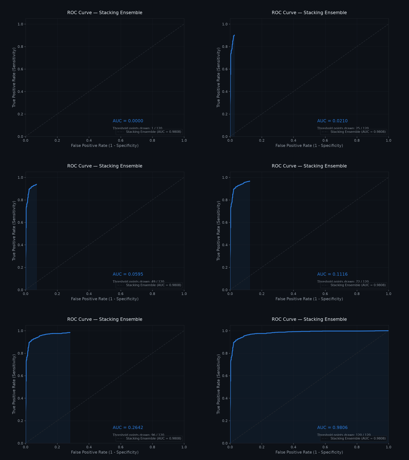
The model achieves a test AUC of 0.9808 and 94% accuracy on 1,518 held-out candidates, with errors balanced across both classes.

How It Was Built

Data Cleaning and Leakage Removal

The cumulative KOI table was filtered to rows with resolved dispositions (CONFIRMED or FALSE POSITIVE), removing unresolved CANDIDATE entries. Non-numeric and identifier columns were dropped. Missing values were imputed using training-partition medians only, applied identically to the test partition to keep the held-out set statistically clean.

The most consequential cleaning step was feature selection. The following columns were excluded entirely:

Direct leakage: koi_disposition, koi_pdisposition, koi_score, koi_fpflag_nt, koi_fpflag_ss, koi_fpflag_co, koi_fpflag_ec, kepler_name
Vetting pipeline diagnostics: koi_dikco_msky, koi_dicco_msky, koi_fwm_stat_sig and all related centroid and flux-weighted centroid columns
Uncertainty columns: all _err1 / _err2 measurement error columns, which encode missingness patterns correlated with vetting attention rather than planet physics

Rather than maintaining a blacklist (which risks missing unanticipated diagnostic columns), the final model trains on an explicit whitelist of 24 physically interpretable features, described below.

Class Distribution and Imbalance Handling

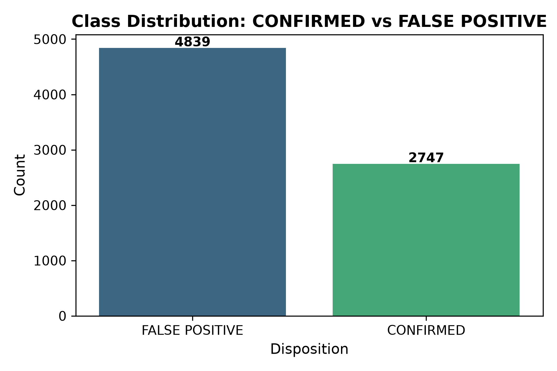
The resolved KOI dataset contains 4,839 FALSE POSITIVE and 2,747 CONFIRMED candidates — a 64/36 imbalance. Two decisions were made in response. First, a stratified train/test split was used to preserve this ratio identically across both partitions. Second, SMOTE-style synthetic oversampling was deliberately avoided: interpolating between existing samples on heavily right-skewed physical quantities such as orbital period, transit depth, and planet radius can generate combinations that are mathematically interpolated but physically impossible — orbital periods that violate Kepler's third law for the given stellar mass, or planet radii that are geometrically inconsistent with the reported transit depth. Stratified splitting and weighted F1 as the primary metric together ensure the model is evaluated fairly across both classes without fabricating data.

Feature Engineering

Seven features were derived from first principles, encoding physical consistency conditions that astronomers apply manually during vetting.

1. Duty Cycle

The fraction of the orbital period during which the planet is in transit:

$$DC = \frac{t_{dur}}{P \times 24}$$

where t_dur is transit duration in hours and P is the orbital period in days. For a circular orbit, the physical upper bound on duty cycle is:

$$DC_{max} \approx \frac{R_\star}{\pi a}$$

where a is the orbital semi-major axis. A transit signal whose duty cycle significantly exceeds this bound given its stated orbital separation and host star size is geometrically impossible as a genuine transit — it would require the planet to spend more time in front of the star than the star's own diameter permits at that orbital distance.

Plain English: If a signal claims a planet is blocking starlight for longer than is physically possible given how far away it orbits, it is almost certainly not a real planet. This feature checks that the timing makes geometric sense.

2. Depth per SNR

$$depth_per_snr = \frac{\delta}{SNR + \varepsilon}$$

where delta is the fractional transit depth in parts per million, SNR is the model signal-to-noise ratio, and epsilon = 1e-5 prevents division by zero. A large transit depth measured with low statistical confidence is fundamentally less trustworthy than a shallower transit detected cleanly. This ratio encodes that joint credibility directly rather than requiring the model to infer it from two separate columns.

Plain English: A faint blur in a noisy photograph tells you much less than a sharp image of a small object. This feature measures how confidently the brightness dip was actually detected, relative to how deep it was.

3. Transit-Derived Stellar Density Consistency (rho_ratio)

From Kepler's third law, the mean stellar density can be derived purely from the transit light curve geometry (Seager & Mallén-Ornelas 2003):

$$\rho_{transit} \propto \frac{(a/R_\star)^3}{P^2}$$

The same quantity estimated from stellar spectroscopy is:

$$\rho_{catalog} \propto \frac{M_\star}{R_\star^3}$$

The ratio of these two estimates:

$$rho_ratio = \frac{\rho_{transit}}{\rho_{catalog}}$$

For a genuine planet transiting its stated host star, rho_ratio ≈ 1. A background eclipsing binary is not orbiting the target star — its implied orbital geometry is inconsistent with the catalogued stellar parameters, producing a ratio that deviates significantly from unity. This test has been used by NASA itself to eliminate false positive candidates at scale.

Plain English: Every transit implies something about what kind of star the transiting object is orbiting. If you calculate what the star must look like given the transit timing, and that description does not match the star you are actually looking at, something is wrong. A real planet matches its star; an impostor does not.

4. Transit Duration Consistency (duration_ratio)

The maximum physically possible transit duration for a central transit at orbital separation a around a star of radius R_star is:

$$t_{\max} \approx \frac{R_\star \cdot P}{\pi a}$$

The observed-to-expected duration ratio:

$$duration_ratio = \frac{t_{obs} / 24}{t_{max}}$$

Values significantly above 1 indicate the transit lasts longer than the stellar diameter physically permits at that orbital distance — a hallmark of grazing eclipsing binaries and background blends where the true occulting object is much larger than a planet.

Plain English: There is a hard limit on how long a transit can last given the size of the star and how far away the orbiting object is. If a signal lasts longer than that limit, the object causing it cannot be what it claims to be.

5. Radius Regime (radius_regime)

The Fulton et al. (2017) radius gap — a well-established deficit of planets with radii between 1.5 and 2.0 Earth radii — divides the confirmed planet population into physically distinct groups. False positives, dominated by stellar-sized and sub-stellar objects, populate a completely different part of radius space.

Regime	Range	Class
0	R_p < 1.5 Re	Rocky super-Earth
1	1.5 <= R_p < 2.0 Re	Fulton gap
2	2.0 <= R_p < 4.0 Re	Sub-Neptune
3	4.0 <= R_p < 12.0 Re	Giant planet
4	R_p >= 12.0 Re	Stellar-sized — likely false positive

Plain English: Real planets come in predictable sizes that cluster into distinct families. Objects that come out at stellar sizes are almost always two stars eclipsing each other, not a planet at all. This feature tells the model which size family each candidate belongs to.

6. Orbital Velocity Proxy (v_orb_proxy)

From the vis-viva equation for a circular orbit:

$$v_{orb} \propto \sqrt{\frac{M_\star}{a}}$$

Transit duration scales inversely with orbital velocity — faster-moving objects produce shorter transits. This feature provides the model with an independent velocity estimate that can be cross-checked against the observed transit duration without directly reusing the duration column.

Plain English: Objects orbiting close to their star move faster and cross it more quickly. This feature tells the model how fast each candidate should be moving, which is another way to check whether the transit duration makes sense.

7. Habitable Zone Distance (hz_distance)

Stellar luminosity scales from the Stefan-Boltzmann law as:

$$L_\star \propto R_\star^2 \left(\frac{T_{eff}}{T_\odot}\right)^4$$

The habitable zone midpoint scales as:

$$a_{HZ} \propto L_\star^{0.5}$$

giving the dimensionless orbital environment parameter:

$$hz_distance = \frac{a}{\sqrt{L_\star}}$$

This captures where in the stellar radiation environment each candidate sits — a physically meaningful orbital context that differs systematically between populations of confirmed planets and false positives.

Plain English: Each star has a region around it where liquid water could exist on a planet's surface — not too hot, not too cold. This feature measures how far each candidate sits from that region, providing context about what kind of orbital environment it inhabits.

Model Architecture

A stacking ensemble combining five tree-based base learners with a logistic regression meta-learner:

Component	Configuration
Random Forest	100 estimators
XGBoost	100 estimators, lr = 0.05
Gradient Boosting	100 estimators
LightGBM	100 estimators, lr = 0.05
CatBoost	100 estimators, lr = 0.05
Meta-learner	Logistic Regression (C = 0.1)

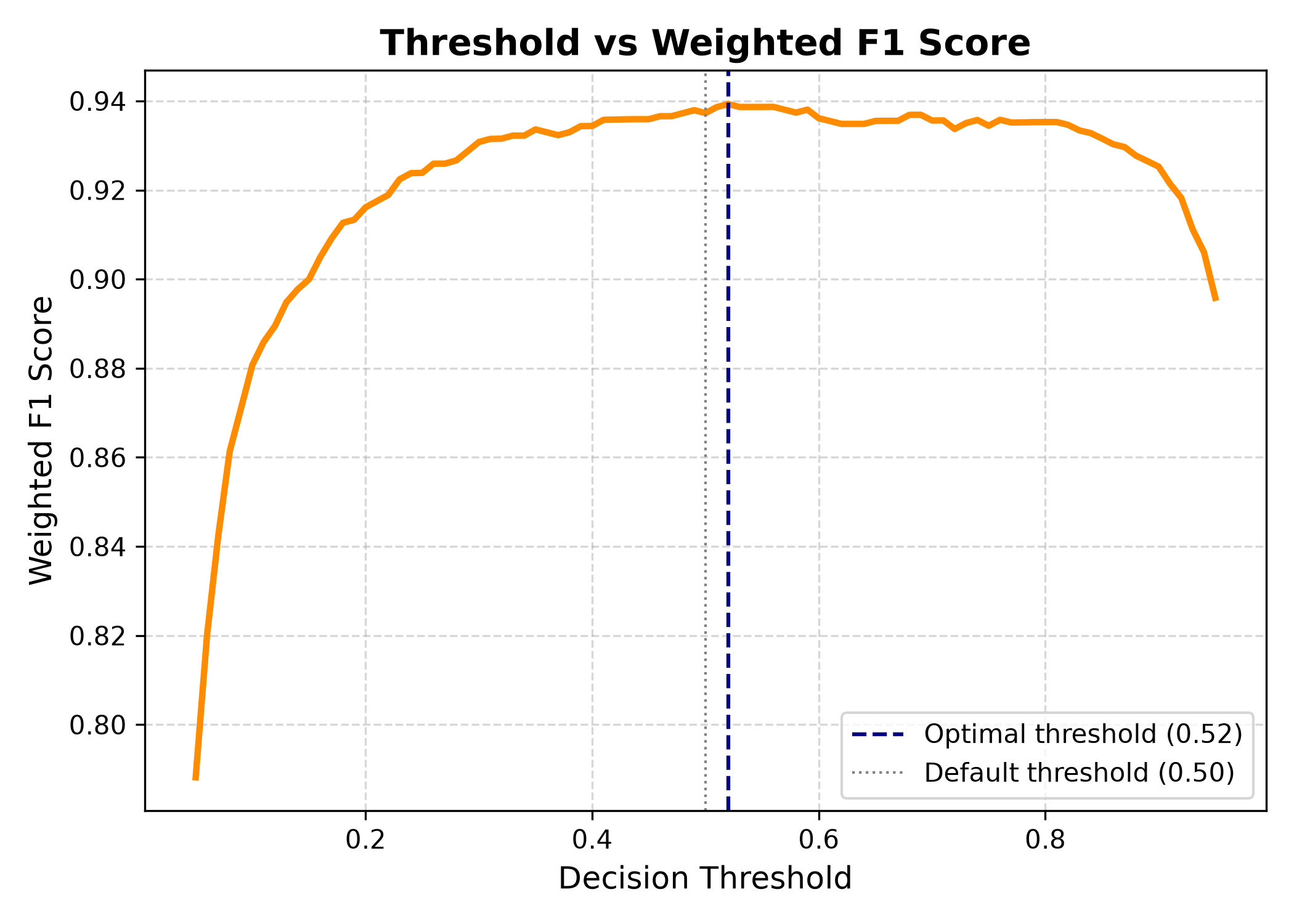
StackingClassifier uses 5-fold cross-validation internally to generate out-of-fold base-model predictions for the meta-learner, preventing in-sample leakage into meta-learner training. The meta-learner's task is linear — it learns the optimal weighting of five already-calibrated probability estimates — making logistic regression the correct choice over a more complex algorithm. Decision threshold was tuned from the default 0.5 to 0.52 via weighted F1 sweep across the full 0.05 to 0.95 range.

Results

Metric	CONFIRMED	FALSE POSITIVE	Overall
Precision	0.95	0.92	0.94 weighted
Recall	0.96	0.91	0.94 weighted
F1-Score	0.95	0.92	0.94 weighted
Accuracy			0.94
Testing AUC			0.9808
Training AUC			0.9974

The train/test AUC gap of 0.0166 is narrower than the 0.0214 gap on the baseline feature set, confirming the engineered features generalize rather than overfit.

Ablation Study — Leakage vs Physics-Only

To quantify the exact cost of removing vetting pipeline diagnostics, the full stacking ensemble was retrained twice: once with the centroid-offset and flux-weighted-centroid columns included (koi_dikco_msky, koi_dicco_msky, koi_fwm_stat_sig, koi_fwm_sdec_err, koi_fwm_srao_err), and once on the physics-only whitelist used in the final model.

Setting	Testing AUC	Weighted F1
With vetting diagnostics included	0.9954	0.9737
Physics-only whitelist (final model)	0.9808	0.9393
Difference	−0.0146	−0.0344

The vetting diagnostic columns inflate AUC by 0.015 and F1 by 0.034. These columns are outputs of the same Kepler disposition pipeline that assigned the labels — including them means the model is partially decoding the answer rather than learning from physical evidence. The final model accepts this performance cost deliberately. A 0.9808 AUC achieved from transit physics alone is a meaningfully stronger scientific result than 0.9954 achieved by partially reading the label back from the feature set.

Why Binary Classification

The KOI table contains three disposition values: CONFIRMED, FALSE POSITIVE, and CANDIDATE. This project frames the problem as binary — CONFIRMED vs FALSE POSITIVE only — for a specific methodological reason. CANDIDATE rows are KOIs that have not yet cleared NASA's confirmation threshold: they are genuinely unresolved cases whose ground truth label does not exist yet. Training a classifier on CANDIDATE rows as a third class would mean learning from observations whose correct label is unknown, which is not a supervised learning problem — it is label noise by definition. The binary framing trains and evaluates only on cases where the ground truth is settled, producing a model whose accuracy estimates are meaningful rather than contaminated by inherently ambiguous examples.

Visualizations And Graphing

ROC Curve

AUC of 0.9808 with true positive rate exceeding 0.90 before the false positive rate reaches 0.10. The steep upper-left rise reflects strong class separation at conservative decision thresholds — the model is highly confident on the candidates it classifies as planets, reserving uncertainty for the genuinely ambiguous borderline cases.

Feature Importance

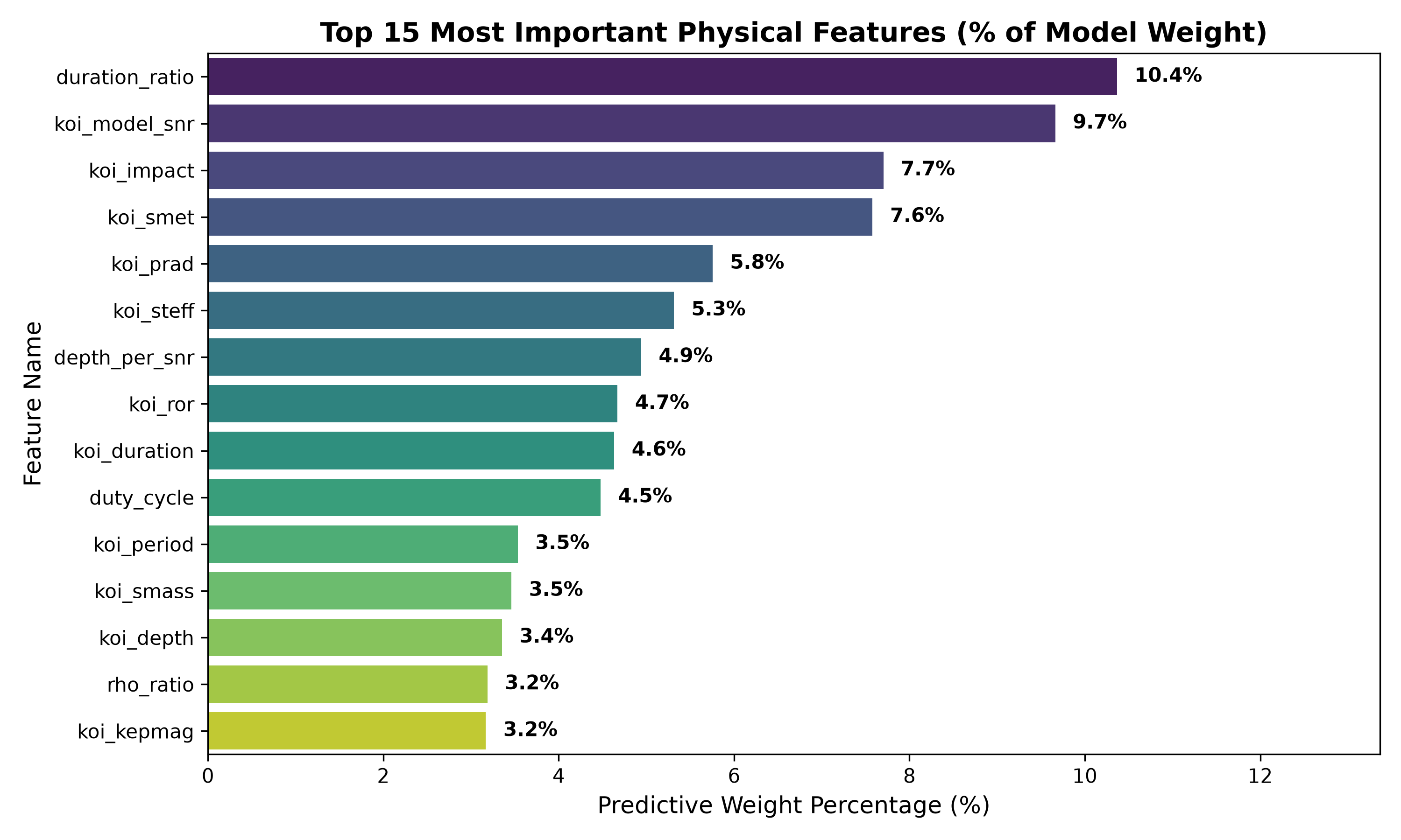
duration_ratio — a feature derived from orbital geometry with no direct equivalent in the raw KOI table — is the single strongest predictor at 10.4%, outperforming every raw measurement column including SNR and planet radius. Two further engineered features (depth_per_snr, rho_ratio) appear in the top 15. No vetting pipeline diagnostic appears anywhere in the ranking.

SHAP Summary

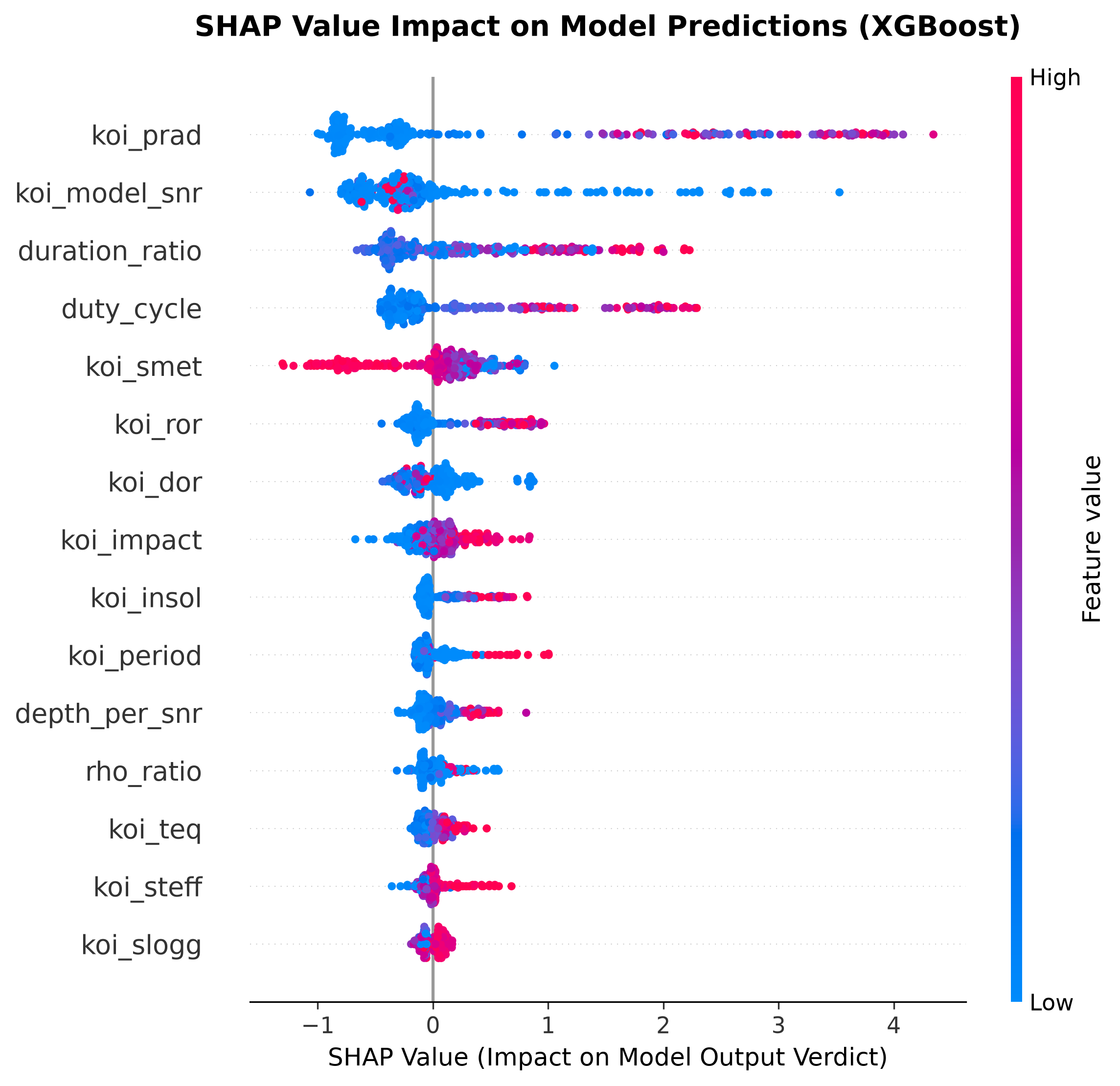
SHAP values confirm both the direction and consistency of each feature's effect at the individual prediction level. High koi_prad values push predictions strongly toward CONFIRMED, extending past SHAP +4 for the largest candidates. koi_smet shows characteristic bidirectional negative contributions at both metallicity extremes, consistent with the nonlinear planet-metallicity relationship. duration_ratio contributes positively for candidates with geometrically self-consistent transit durations. Every directional pattern aligns with established astrophysical reasoning.

Confusion Matrix

	Predicted CONFIRMED	Predicted FALSE POSITIVE
True CONFIRMED	497	53
True FALSE POSITIVE	42	926

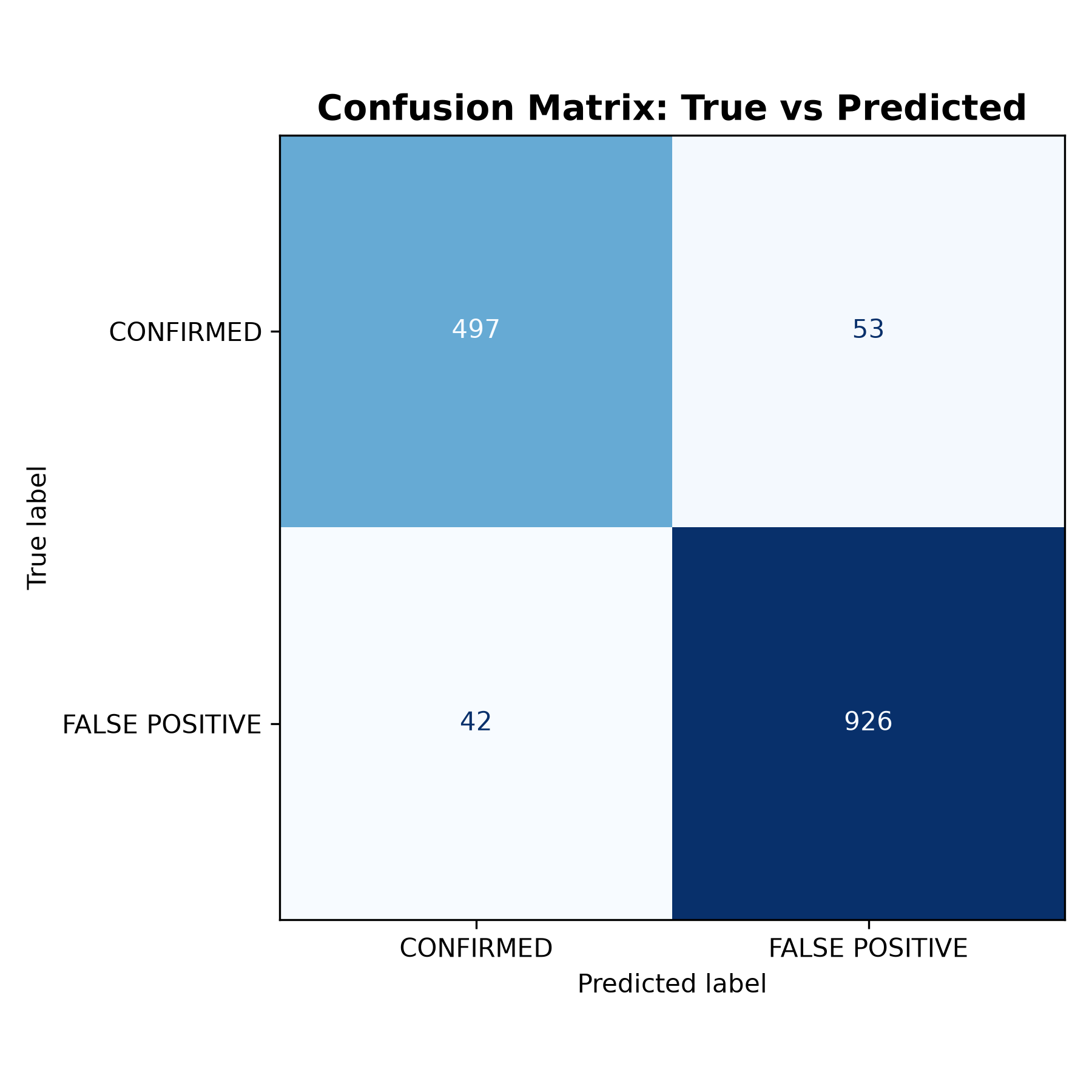
1,423 of 1,518 test samples correctly classified. The physics-derived engineered features reduced false-positive misclassifications by 25% compared to the baseline model (42 vs 56), with no equivalent degradation in planet recall, indicating the new features specifically improved impostor detection.

Correlation Heatmap

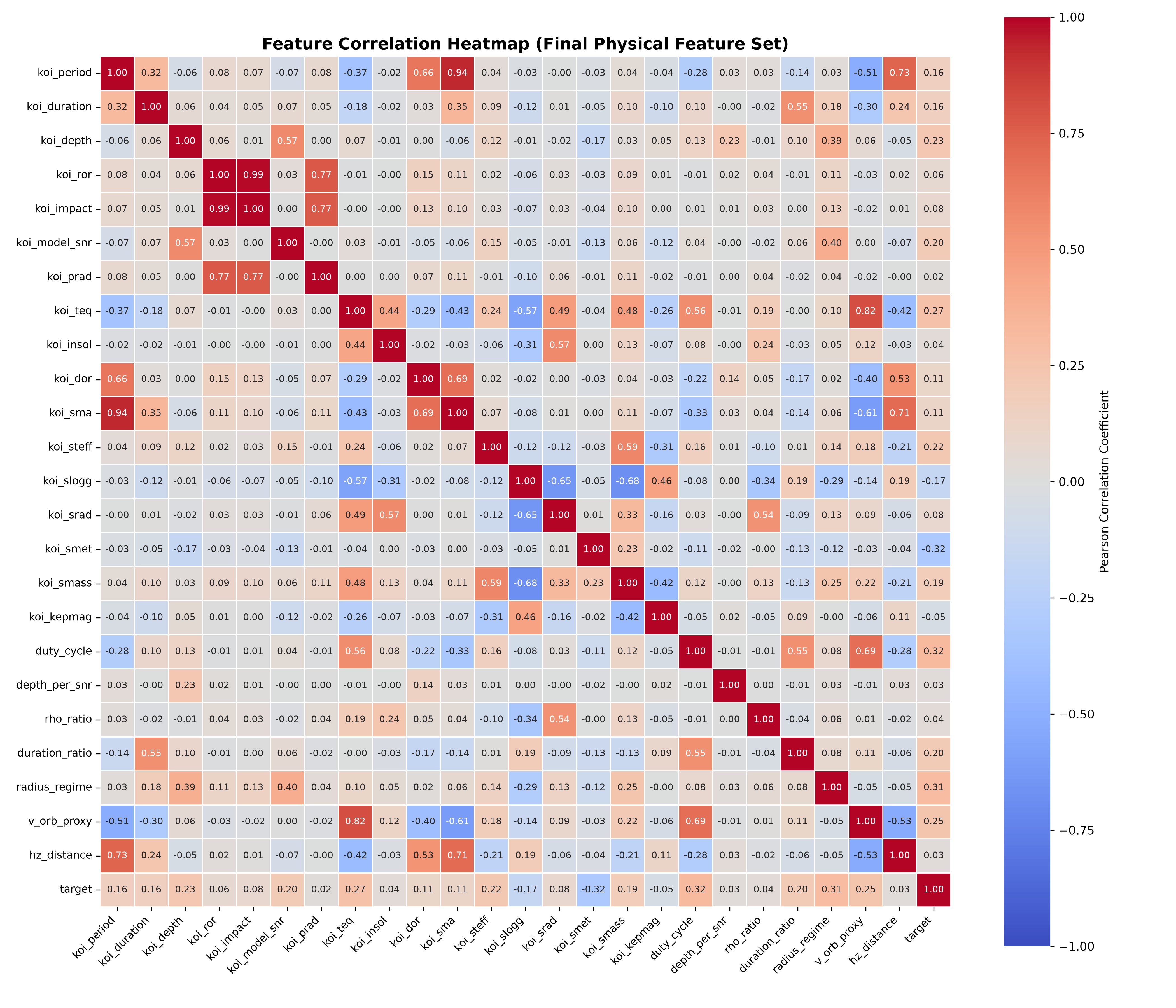
koi_period / koi_sma correlation of 0.94 and koi_ror / koi_impact correlation of 0.99 reflect expected physical relationships from Kepler's third law and transit geometry — not leakage. No engineered feature exceeds 0.55 Pearson correlation with any raw input column, confirming independent signal capture. koi_prad has only 0.02 linear correlation with the target yet carries 5.8% of model weight, demonstrating that its relationship with disposition is nonlinear and only recoverable by tree-based methods.

Precision-Recall Curve

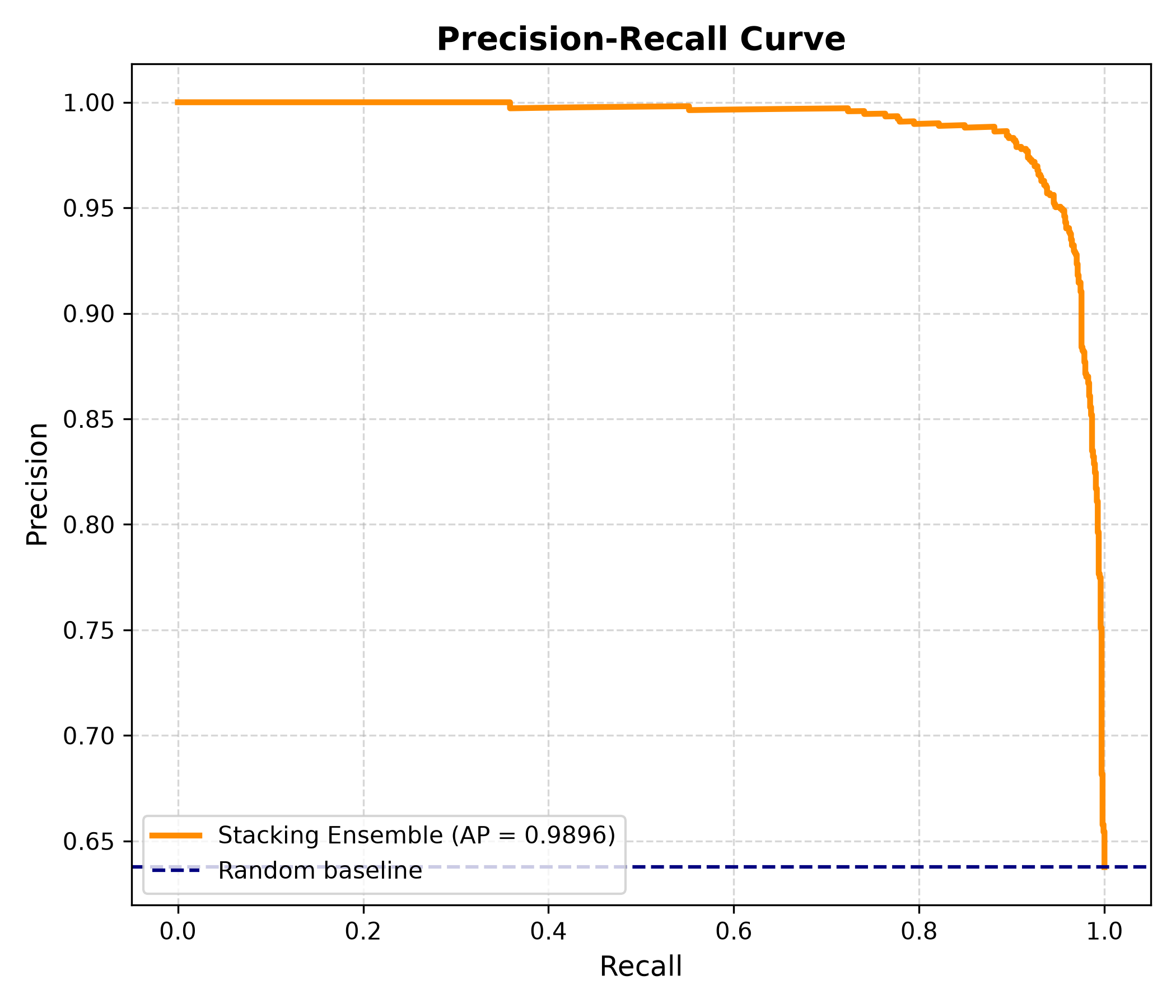
Average Precision (AP) of 0.9896. The curve maintains precision above 0.99 across recall values up to approximately 0.90, meaning the model correctly identifies nearly all confirmed planets before beginning to trade precision for recall. The random baseline sits at 0.64 — the ratio of the majority class — making the gap between the model and baseline visually immediate. PR curves are more informative than ROC curves under class imbalance, since they directly reflect performance on the minority (CONFIRMED) class rather than being inflated by the large number of true negatives in the FALSE POSITIVE class.

Threshold vs Weighted F1

The sweep across all thresholds from 0.05 to 0.95 shows a broad plateau of strong F1 performance between 0.35 and 0.75, with a clear peak at 0.52. The default threshold of 0.50 achieves 0.9373 weighted F1 — only 0.002 below the optimal 0.9393 at 0.52 — confirming the model is already well-calibrated and that the threshold tuning is a refinement rather than a correction. The sharp drop below 0.15 reflects the cost of predicting almost everything as CONFIRMED, while the gradual decline above 0.75 reflects increasing false negatives as the model becomes overly conservative about planet confirmation.

What the Model Learned

Feature importance and SHAP analysis converge on the same conclusion: the model relies on exactly the three checks an experienced astronomer applies when manually vetting a KOI.

First, is the implied object actually planet-sized? koi_prad and radius_regime together encode this check. The Fulton gap encoding alone carries strong linear correlation (0.31) with the target, confirming that the population-level radius structure discovered by Kepler is detectable and discriminating in this dataset.

Second, does the transit's shape and timing make geometric sense? duration_ratio at 10.4% model weight — the top feature — captures exactly this. A transit duration inconsistent with the orbital geometry given the host star's size is the clearest indicator of an impostor. duty_cycle and rho_ratio encode related geometric consistency conditions from different physical angles.

Third, is the detection statistically convincing? koi_model_snr at 9.7% and depth_per_snr together encode detection confidence. High-SNR detections push strongly toward CONFIRMED in the SHAP plot; borderline-SNR candidates correctly attract uncertainty.

The absence of any vetting pipeline diagnostic in the top fifteen features is not a negative result — it is the main result. It demonstrates that 0.9808 AUC is achievable from transit physics alone, without any information from the same process that assigned the labels being predicted.

Explaining the Predictions to a Non-Technical Audience

Every night, thousands of stars are watched for one thing: a repeating dimming, like a shadow crossing a lamp. A real planet produces a shadow that is small, consistent, and perfectly timed to its orbit. But many things can fake that shadow. Another star eclipsing its partner from across the galaxy can produce an identical pattern. A smudge of blended starlight can dim and brighten on a schedule that looks orbital. Even an instrument glitch can repeat.

The model checks four things about every candidate signal. First: is the object the right size to be a planet, not a star? Second: does the timing of the dimming make sense given how far out the object orbits — because there is a hard geometric limit on how long a transit can last? Third: does the stellar density implied by the transit's shape match what we know about the actual star it claims to orbit? Fourth: is the detection itself strong and clean, or is it barely distinguishable from noise?

A candidate that passes all four checks is called a likely planet. One that fails any of them — an object too large to be a planet, a transit that lasts longer than the geometry allows, a density mismatch between the transit and the star, or a detection too faint to trust — is flagged as a likely impostor. The model applies these four checks to every candidate simultaneously, getting the answer right 94 times out of 100 on signals it has never seen before.

Challenges

Leakage was invisible until it was obvious. The first model scored 0.99 AUC and appeared to work flawlessly. Examining feature importance revealed that koi_dikco_msky — a centroid-offset statistic the Kepler pipeline computes specifically to flag background eclipsing binaries — was the top predictor, accounting for over 20% of model weight. This is not a physical measurement of the planet; it is a pre-computed false-positive test, a partial copy of the answer key sitting inside the feature set. Systematically identifying and removing every column of this type, then verifying the model still achieved strong performance on a physics-only whitelist, was the hardest and most important part of the project.

The error columns were a subtler trap. Measurement uncertainty columns (_err1, _err2) appear innocuous — they just encode how precisely each measurement was made. But in practice, the quality and completeness of these measurements correlates strongly with how much follow-up vetting attention a candidate received, which in turn correlates with its eventual disposition. They encode not the physics of the planet but the history of the pipeline, and had to be excluded for the same reason as the explicit diagnostic columns.

Deriving physically meaningful features required domain research. The seven engineered features were not found by running automated feature selection — they were derived by researching how astronomers actually vet transit candidates, identifying the geometric consistency conditions they apply, and translating those conditions into computable quantities from the available columns. duration_ratio becoming the model's top feature validated that approach directly.

What's Next

Cross-validation with mean ± std F1 and AUC across 5 folds is the immediate next step, providing statistical confirmation that the results generalize beyond this single train/test split. Cost-sensitive threshold optimization is a natural extension — a missed real planet and a wasted telescope follow-up observation carry genuinely different costs, and the optimal threshold should reflect that asymmetry rather than treating both errors equally. Hyperparameter tuning via RandomizedSearchCV would address the residual 0.0166 train/test AUC gap. Longer term, applying the same leakage-aware, physics-grounded feature engineering to TESS Object of Interest data would test whether the physical reasoning learned on Kepler transfers across missions and instrument epochs — a stronger validation than cross-validation within a single dataset can provide.

Byte Breakers