-
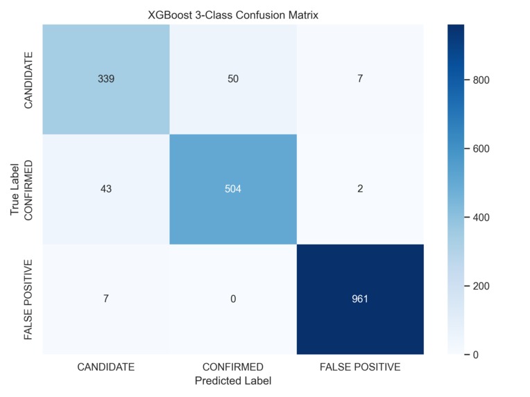
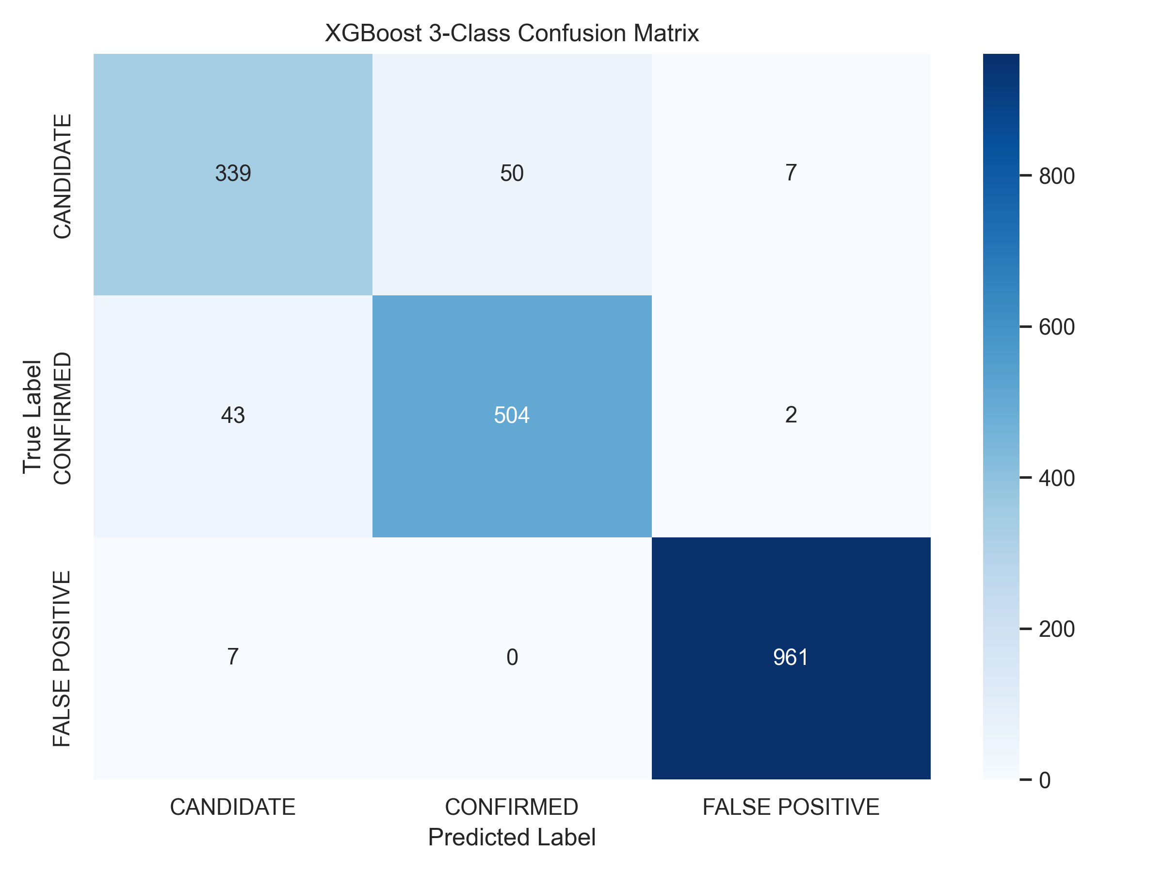
confusion matrix
-
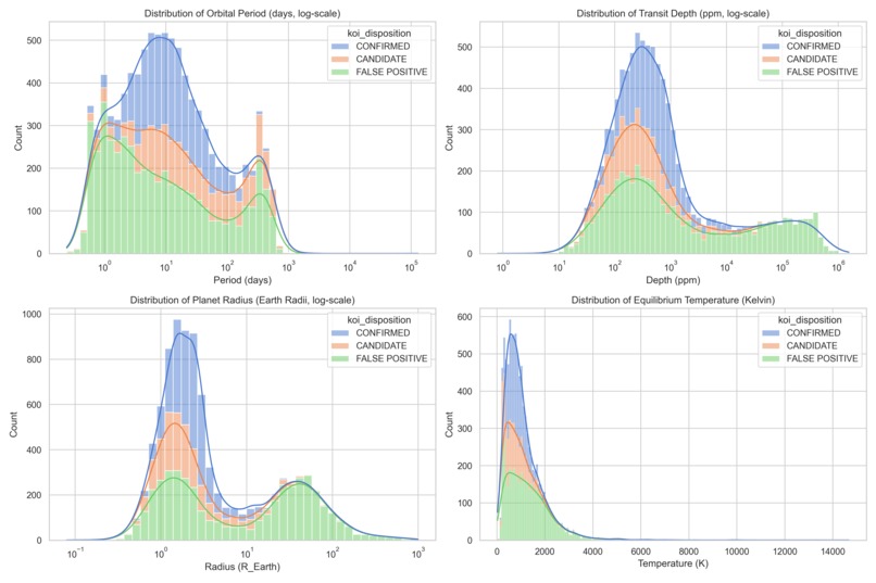
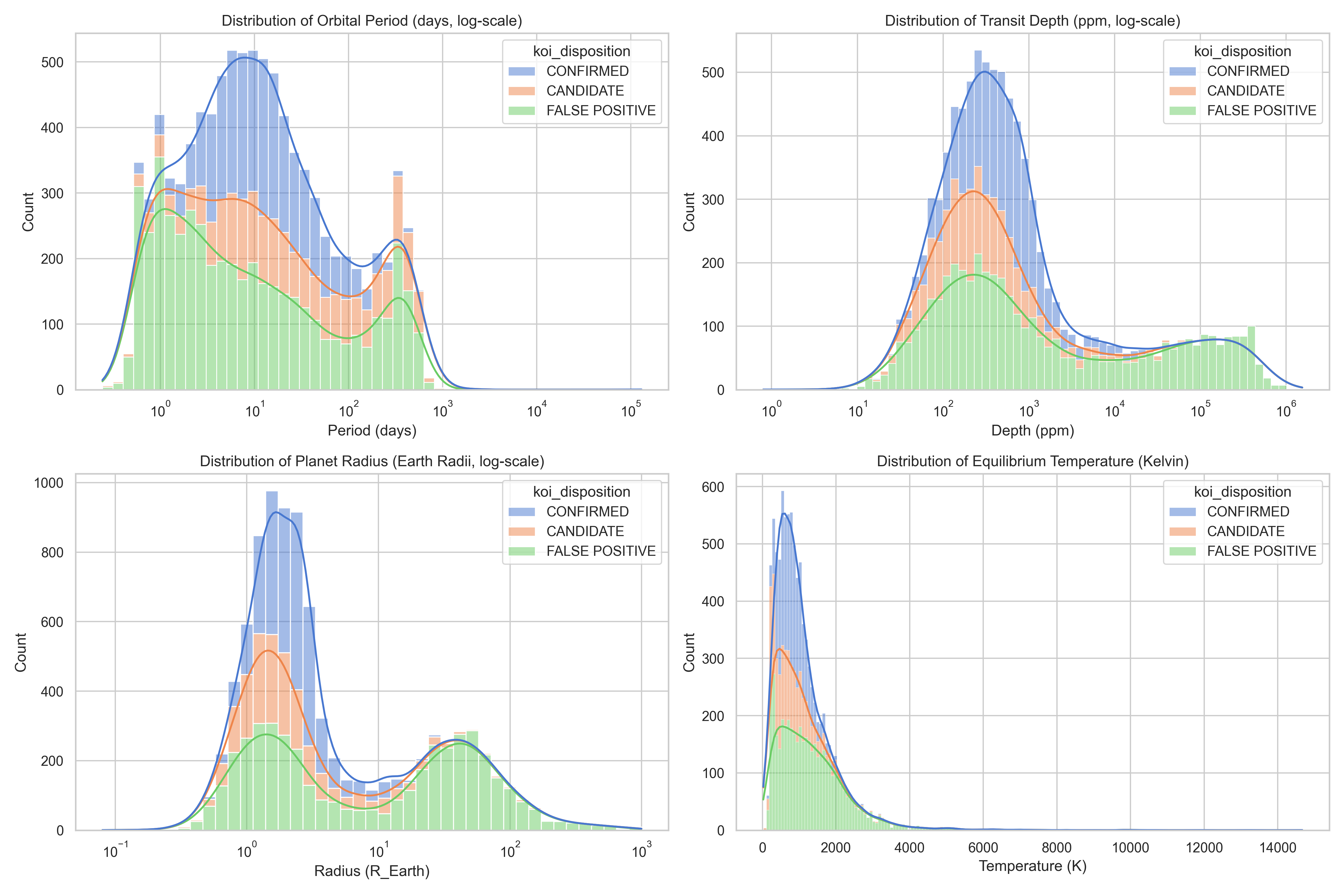
Transit Features
Inspiration Our inspiration stems from a fundamental question: How do we find planets orbiting stars that are trillions of miles away?
Because exoplanets are too small and dim to see directly, space telescopes like NASA's Kepler monitor the slight dimming of starlight that occurs when a planet transits in front of its host star. However, telescope data is extremely noisy—flares, instrument glitches, and eclipsing binary stars mimic these transits, creating thousands of false alarms. We wanted to build an AI-driven vetting pipeline that acts as an automated "assistant astronomer," separating real exoplanet candidates from background noise and stellar false positives using real space telescope data.
What it does The project is a machine learning vetting pipeline that analyzes Kepler Objects of Interest (KOIs) from the NASA Exoplanet Archive. It takes raw photometric and stellar features and classifies them into one of three categories:
CONFIRMED: Actual exoplanets validated by follow-up observations. FALSE POSITIVE: Dimming events caused by eclipsing binary stars, background stars, or instrument glitches. CANDIDATE: Unresolved, transit-like signals that are potential exoplanets but require further study. By automatically filtering out false alarms, this model helps astronomers prioritize which candidate systems to target with expensive ground-based telescopes (like Keck or James Webb), saving years of manual vetting.
How we built it We built the machine learning pipeline in Python using a state-of-the-art data science stack:
Exploratory Data Analysis (EDA): Used matplotlib and seaborn to visualize class distributions and log-scaled transit features (like orbital period, depth, planetary radius, and temperature). Data Cleaning & Target Leakage Prevention: Dropped columns like kepler_name (assigned only after confirmation) and koi_pdisposition (pipeline heuristics) to prevent target leakage. We also removed constant columns and columns with >50% missing values, imputing remaining data using robust median imputation. Feature Engineering: Derived physics-informed features from raw astronomical measurements: Semi-Major Axis (AU): Approximated the planet's orbital distance from the star using Kepler's Third Law: a ∝ ( P years 2 ⋅ M star ) 1 / 3 a∝(P years 2 ⋅M star ) 1/3 . Planet-to-Stellar Radius Ratio ( R p / R s R p /R s ): A direct indicator of transit depth. Transit Fraction: The ratio of transit duration to orbital period. Stellar Density: Approximated from stellar mass and radius ( M s / R s 3 M s /R s 3 ). Quarters Observed Count: Extracted from the Kepler observation binary mask string. Model Training & Selection: Trained and compared three ensemble models (Random Forest, XGBoost, and LightGBM). We evaluated them on both a 3-class problem and a binary classification problem (Confirmed vs. False Positive). Explainability: Extracted global Gini feature importances and computed local and global SHAP (SHapley Additive exPlanations) values to map the physical decision boundaries. Challenges we ran into Target Leakage: The raw NASA data has columns like kepler_name that are only filled when a planet is confirmed. Early model drafts had "100% accuracy" because they simply checked if this name was missing. We had to carefully identify and prune these columns to ensure our model generalizes to new, unconfirmed candidates. Log-Scale Plotting and Noise: Key parameters like transit depth (koi_depth) spans orders of magnitude and includes negative values due to background noise. Standard log-scaling crashed our KDE density plots because you cannot take the logarithm of a negative number. We had to filter out non-positive values specifically for visualizations. The "Candidate" Gray Area: Classifying the CANDIDATE class is significantly harder than a binary clean/dirty classification. Candidates physically look identical to confirmed planets but lack the follow-up data. The model had to learn highly subtle patterns in Signal-to-Noise Ratio (SNR) and orbital characteristics to separate them. Accomplishments that we're proud of Exceptional Performance: Our final XGBoost model achieved 94.30% Accuracy and a 92.31% Macro F1-score on the complex 3-class classification, and our LightGBM model reached 99.93% Accuracy on binary classification. Scientifically Grounded AI: Through SHAP values, we proved that our model actually learned real physics. For example, it learned that objects with a radius larger than 20–30 Earth radii are virtually always eclipsing stars (False Positives), mirroring real astrophysical bounds. Reproducibility: The entire workflow is compiled into a single, clean, and documented Jupyter Notebook that runs top-to-bottom without a single warning or error.
Built With
- artificial-intelligence
- astronomy
- data-analysis
- data-cleaning
- data-science
- feature-engineering
- jupyter-notebook
- lightgbm
- machine-learning
- numpy
- pandas
- python
- random-forest
- scikit-learn
- shap
- space-science
- xgboost


Log in or sign up for Devpost to join the conversation.