-
-
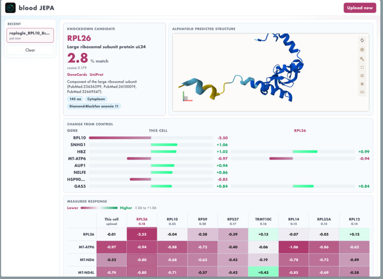
dashboad
-
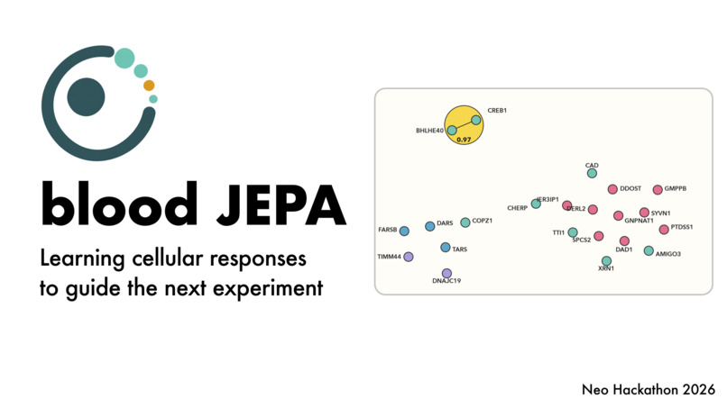
blood JEPA
-
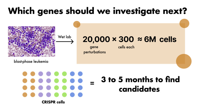
Which genes should we investigate next?
-
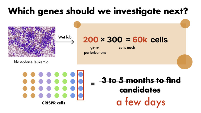
Our advantage
-
Our approach
-
How our model performed
Inspiration
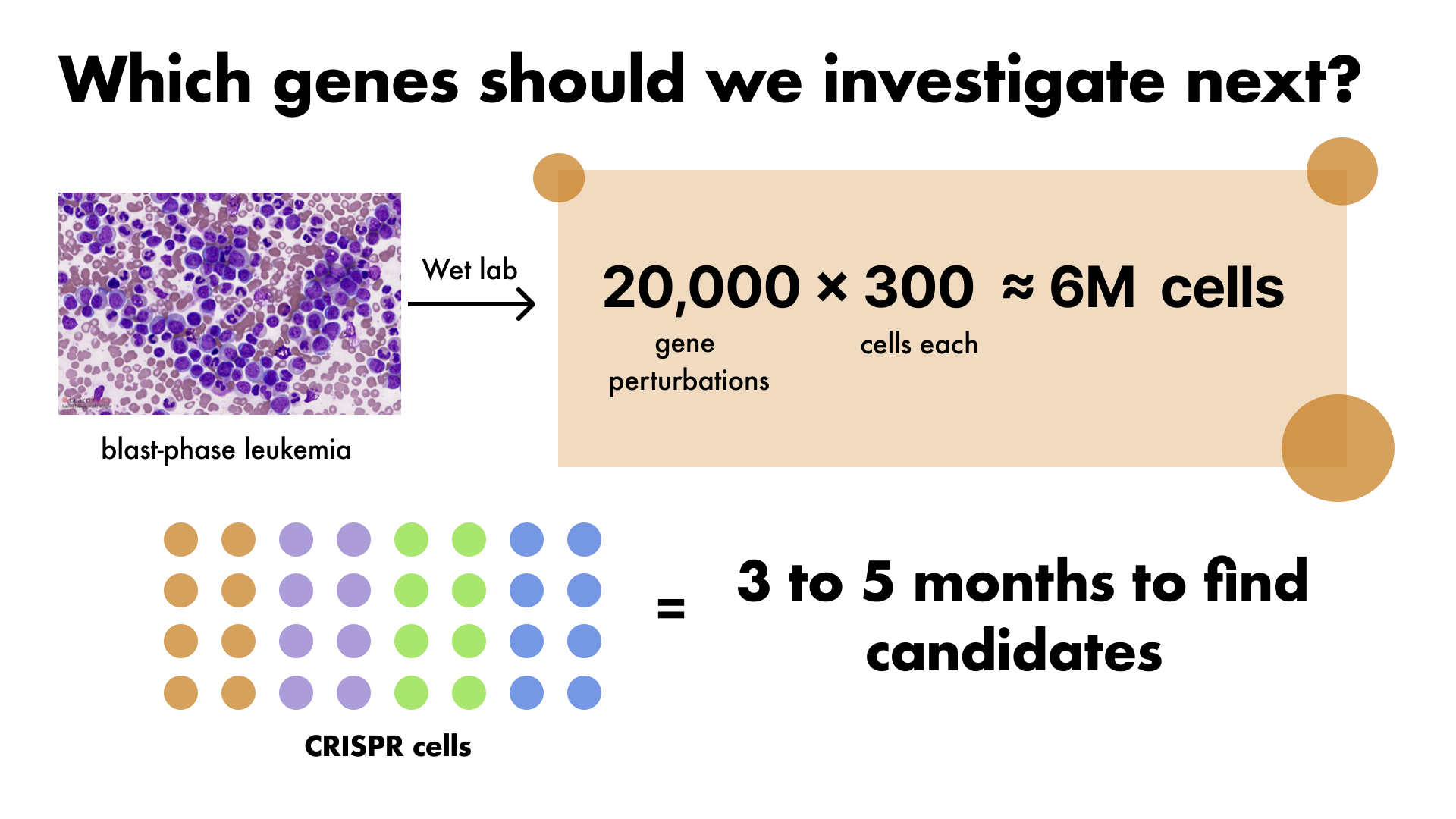
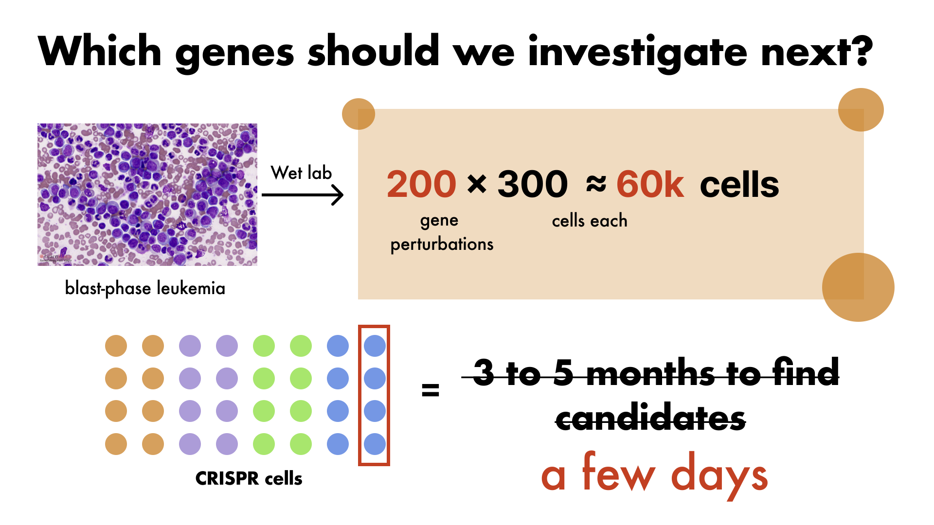
We were really curious about world models and applying them to fields that they traditionally haven’t been applied to. After researching how wet labs go about selecting potential gene candidates for treatments for diseases like leukemia, we realized that choosing which genes to screen relies heavily on intuition and literature review, but over 80% of genes lack this kind of data/insight. To find which genes matter to treat a disease like blast-phase leukemia, you suppress genes one at a time and record the state of the cell. But there are a total of roughly 20,000 genes and you need around 300 cells per gene just to average out single-cell noise in this example. A complete screen comes to about 6 million individually sequenced cells and realistically takes 3 to 5 months in a wet lab. We wanted to see if we could improve this process by introducing novel machine learning techniques such as cellular embeddings, gene transformers, and contrastive learning.
What it does
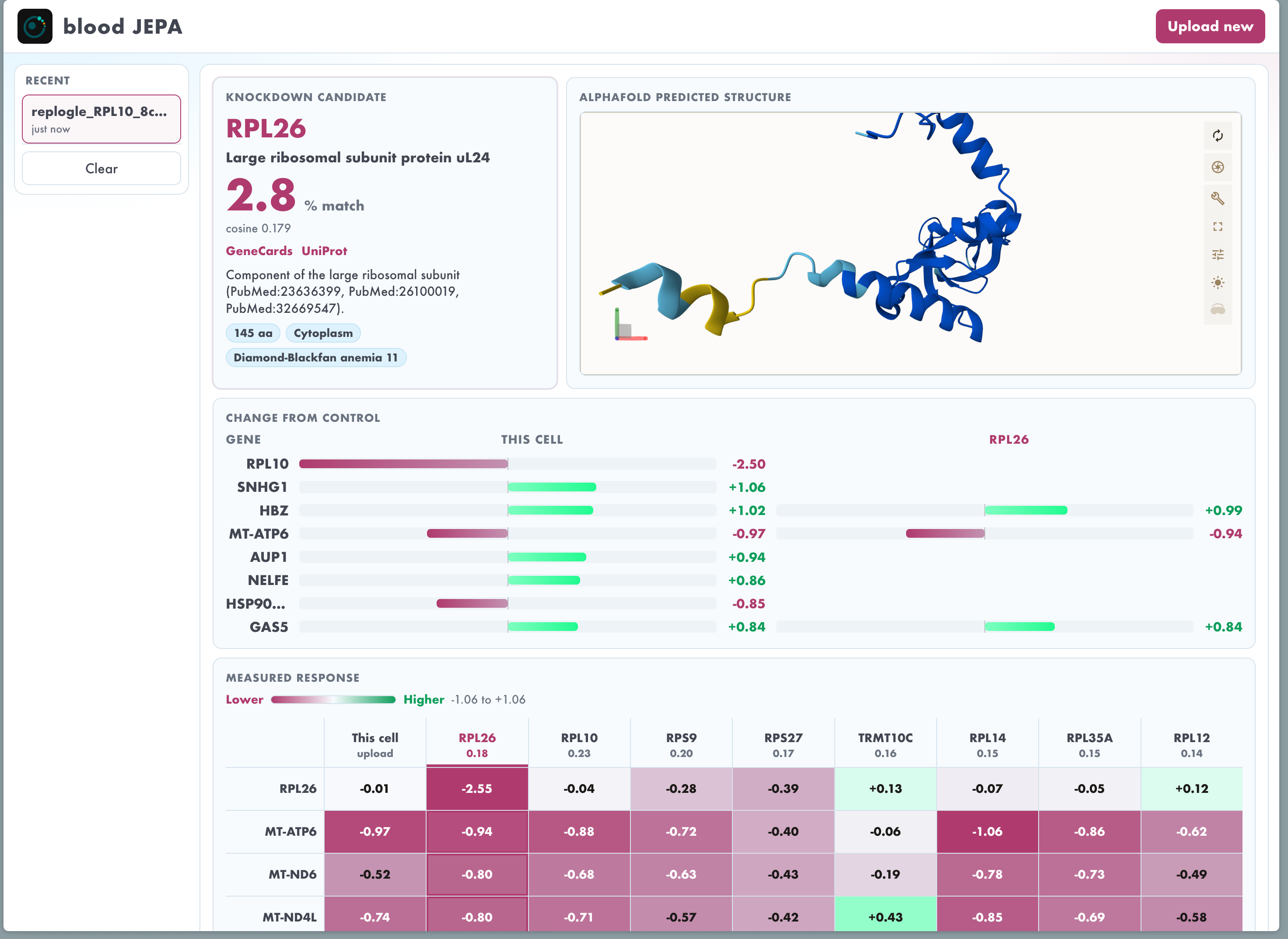
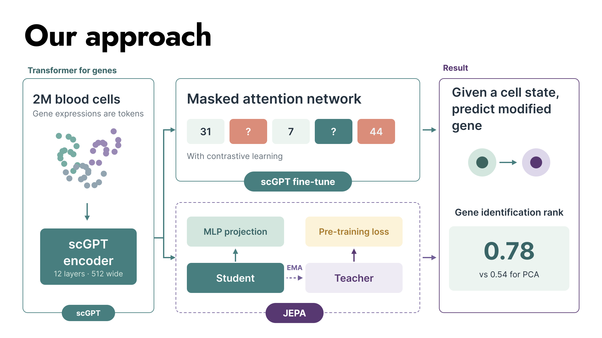
bloodJEPA takes a measured cell state and tells you which modified gene most likely produced it.
A CRISPR researcher gives it a cell profile, either from an experiment they have already run or a state they are trying to engineer toward, and the model returns a ranked list of candidate genes with a probability score against each one. The candidate genes are the ones that express the behavior that we want (ie weakening leukemia cells)
How we built it
We began by reading the literature and reimplementing Cell-JEPA from the paper text, since the method has no public code or checkpoints to work from.
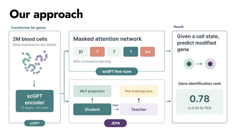
The base model. We started from public scGPT, a transformer that reads a cell the way a language model reads a sentence, where every gene becomes a token carrying its identity and its expression level. We continued pre-training it on 2 million blood and bone-marrow cells from the CELLxGENE Census, and separately trained matched models from scratch on 814,000 kidney cells to match the paper’s setup.
The JEPA objective. On top of that we built the method itself, in which a student network sees a cell with some values hidden and has to predict a teacher’s embedding of the complete cell, where the teacher is an exponential moving average of the student and never receives gradients.
Post-training/Fine-tuning and evaluation. This is where most of our gains came from. The paper scores models on how well they reconstruct expressions, but a researcher actually wants to know which knockdown caused a given response.
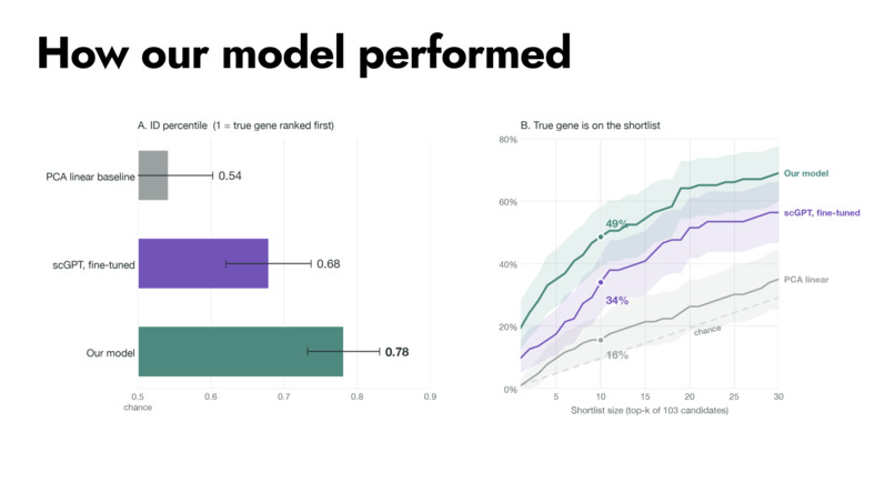
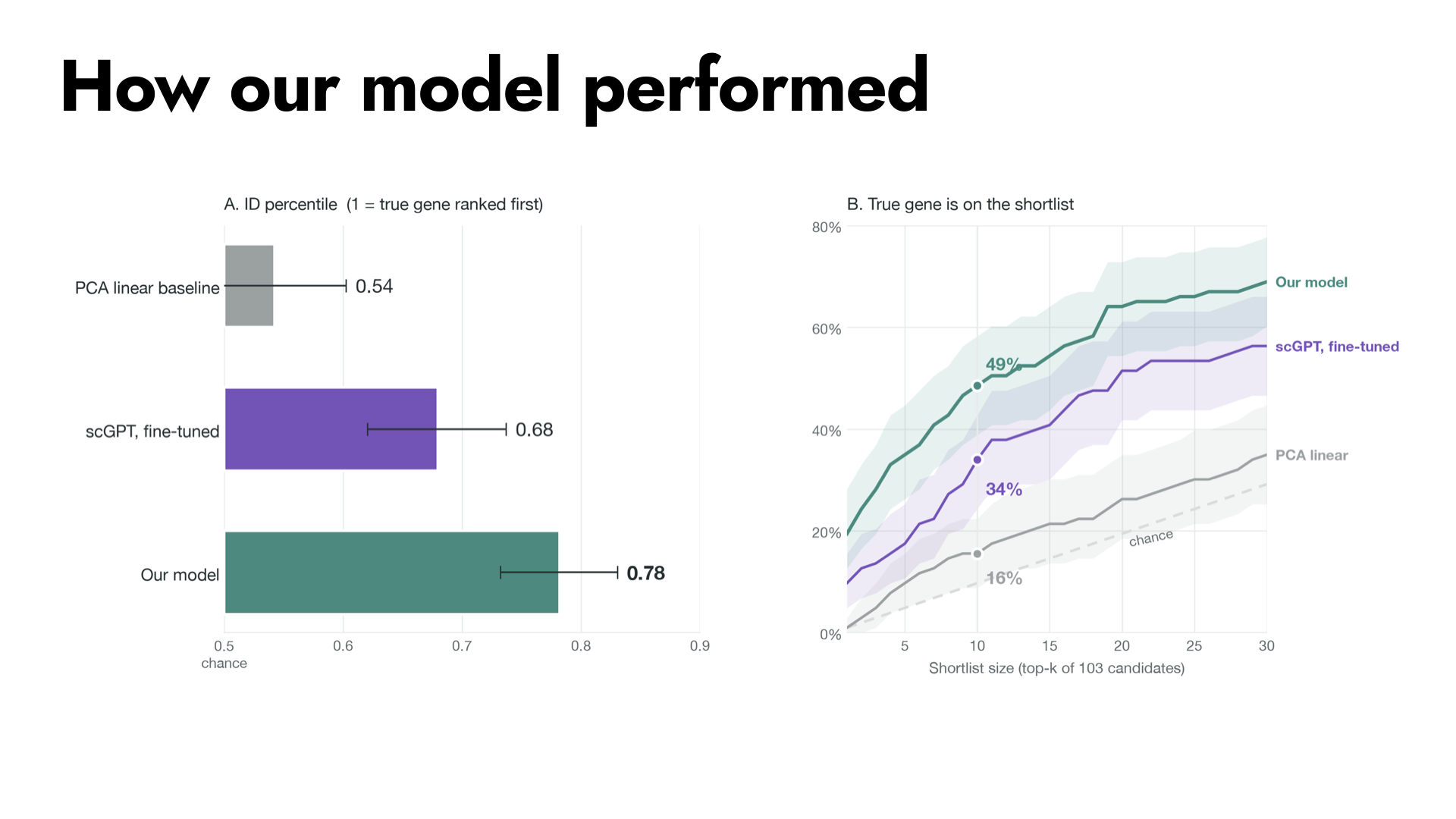
Plain fine-tuned scGPT already beats the standard PCA baseline (0.68 vs 0.54 ID percentile) at this. To improve it, we explored a bunch of things like contrastive loss, which pushes each gene’s predicted response away from all the others, starting from a blood-adapted model, and averaged two seeds. That got us to 0.78 (ID percentile), with the right gene in the top 10 half the time (49% vs 16% for PCA). Those post-training changes ended up mattering a lot and led to significant improvements.
- JEPA Experiments. One of the first tweaks we made was the target the student has to predict. The paper asks it to predict a single pooled summary of the whole cell, so alongside that we implemented a centred version borrowed from Meta’s vision world model DINO, which subtracts a running average of recent targets so the model has to explain what makes each cell different rather than what every cell shares; and an I-JEPA-style version that predicts embeddings of the individual hidden genes rather than one vector for the cell. We also tried to tweak what gets hidden in the JEPA objective. The default is a random scatter of genes, which we suspected was too easy, so we also built masking by whole co-expression gene programs. Another thing we tweaked was how much gets hidden. We swept the masking ratio from the paper’s fifteen percent up through thirty, fifty, and eighty, to see if different masking ratios were optimal.
Accomplishments that we’re proud of
We beat PCA and the industry frontier in identifying which genes to target to reach a given cell state.
We were able to reproduce Cell-JEPA from the paper alone.
Challenges we ran into
The biggest challenge we ran into was that our training of JEPA did not produce statistically better results than the simpler fine-tuned scGPT model. Some of the tweaks to training JEPA that we tried included masking whole co-expression programs rather than just randomly selected genes and sweeping the masking ratio from 15% to 80%, among others, none of which produced statistically significant results. To investigate why JEPA seemed to be failing in this use case, we learned that JEPA’s whole mechanism is learning features that survive a corrupted view, which means discarding fine detail. A knockdown is fine detail: a small shift inside one cell type. We measured it directly: in scGPT’s embedding space you identify the right knockdown 93% of the time; after JEPA training, 68%, with 8× less separation between knockdowns. The property that wins cell-type clustering is the same one that loses perturbation retrieval.
What we learned
We learned to score the model on the decision people actually make. The models that look best on prediction error aren’t actually the ones that find the right gene to target. We learned about contrastive loss, which was super effective (as elaborated on earlier). We learned that although JEPA is good at representations, it wasn’t better at representing cell states and finding the specific necessary knockdowns because of the way that it generalizes.
What’s next for bloodJEPA
- Take the same recipe to tissues that are not blood. Nothing about the method is specific to leukemia. The recipe is to pre-train on a tissue’s cells, fine-tune on whatever perturbations that field has already measured, and then search, and we built the pipeline to be corpus-agnostic from the start. We would go first to the places where cells are precious, and screens are rare, such as induced neurons, engineered T cells, and solid tumour lines, all of which are far less covered than K562.
- Push the contrastive loss to understand near misses. The contrastive objective was the only change that consistently improved results, and it works by pushing every gene that is not the correct answer away from the prediction. However, this fails when two genes in the same complex should produce nearly identical results. We could try to apply a coefficient for the distance between the first gene prediction and the second best to not punish the model as much when gene predictions are closer together. This better represents the real biology and will likely improve the model's performance.
Built With
- computational-bio
- deep-learning
- finetuning
- gene-transformer
- jepa
- machine-learning
- modal
- post-training
- python
- pytorch
- transformer
