-
-
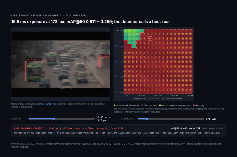
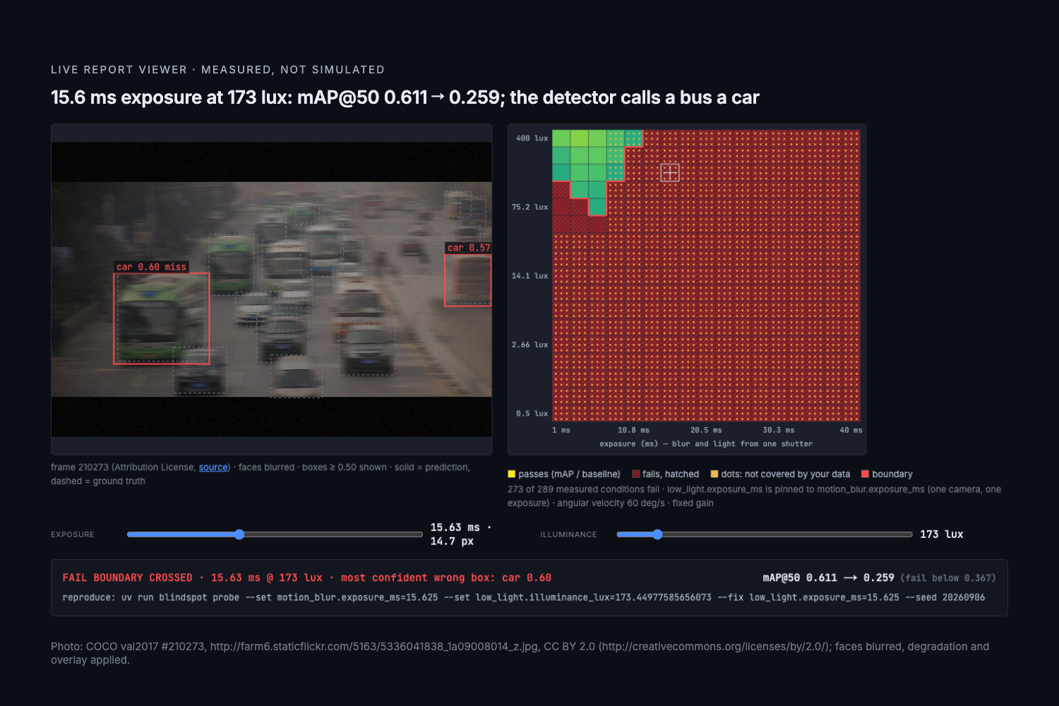
Photo: COCO val2017 #210273 (Flickr), CC BY 2.0; faces blurred, degradation and overlay applied.
-
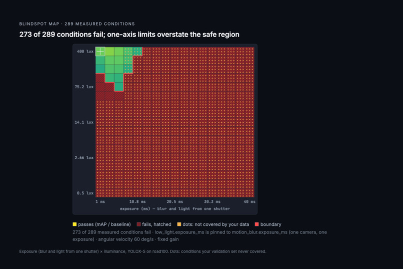
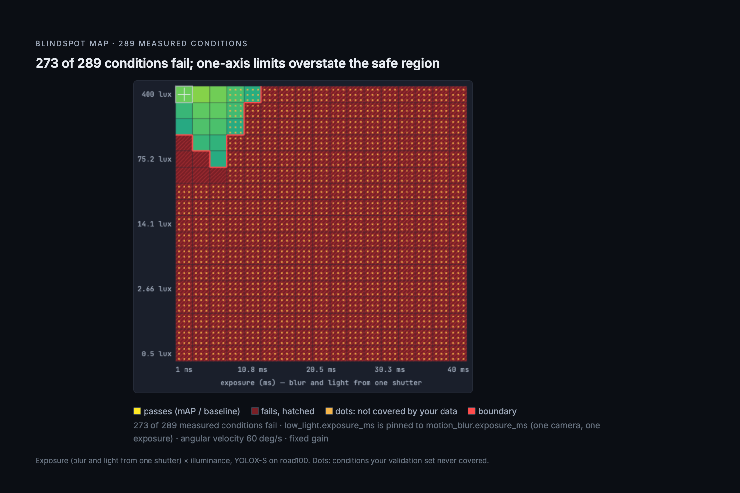
273 of 289 measured conditions fail; one-axis limits overstate the safe region.
-
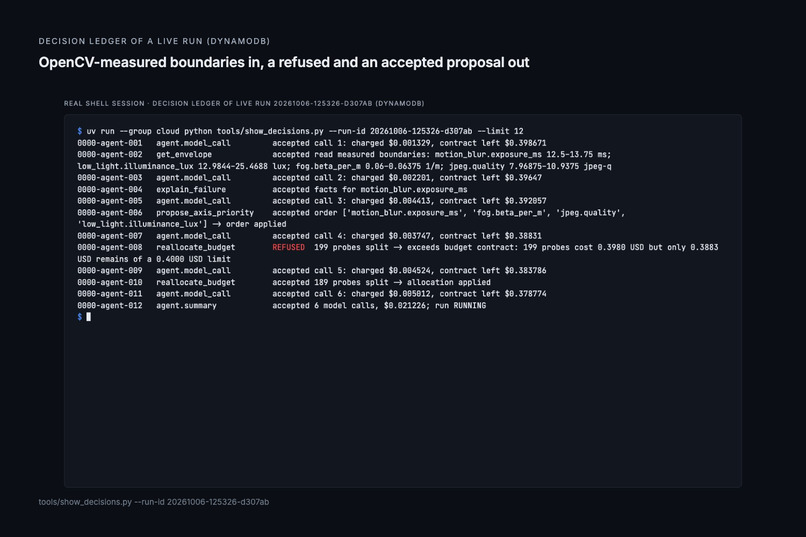
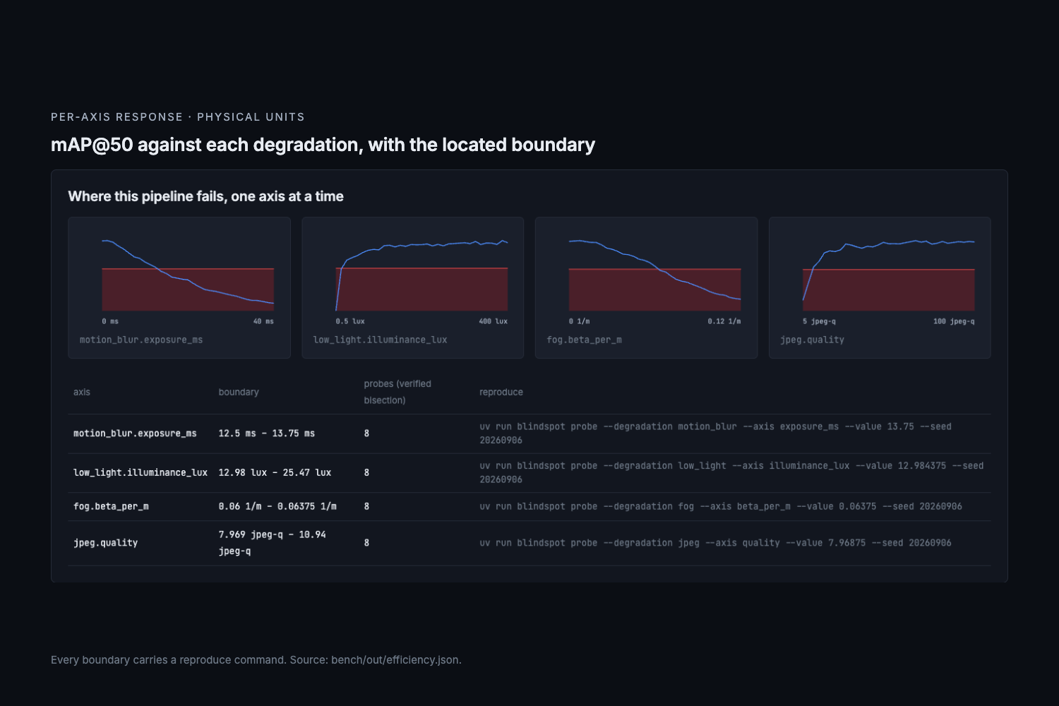
mAP@50 vs each degradation in physical units, with the located boundary and a reproduce command.
-
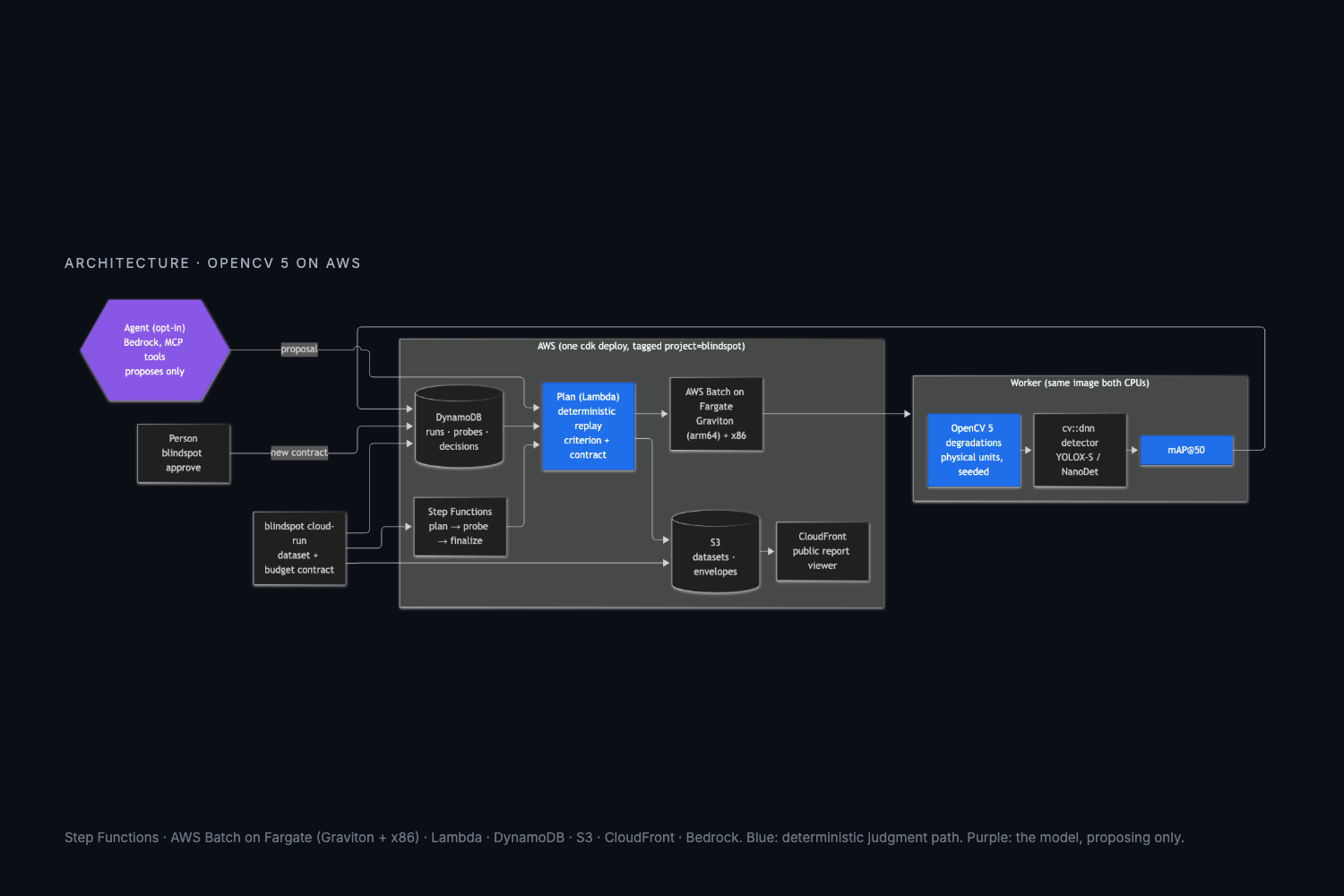
One cdk deploy: Step Functions, AWS Batch on Fargate (Graviton + x86), DynamoDB, S3, CloudFront.
-
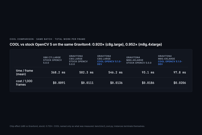
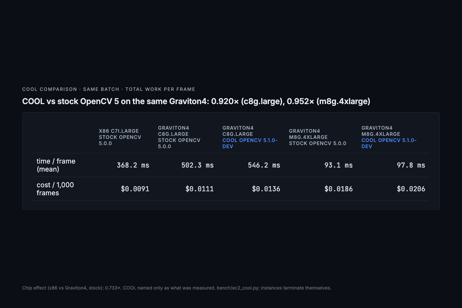
COOL vs stock OpenCV 5 on the same Graviton4: 0.920x and 0.952x. Measured, not integrated.
-
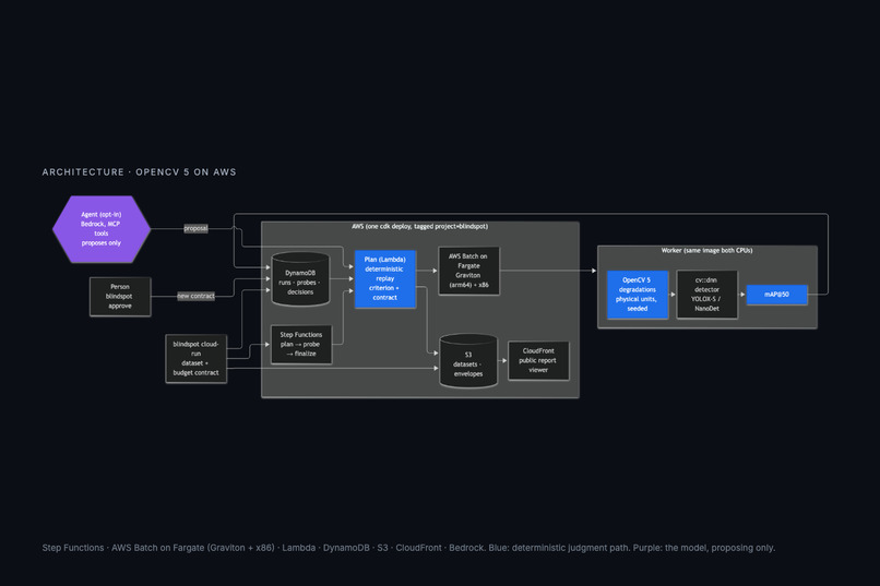
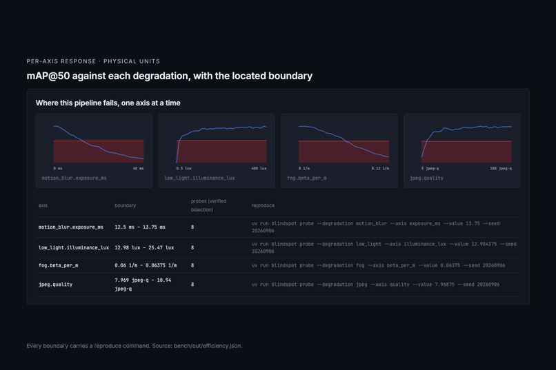
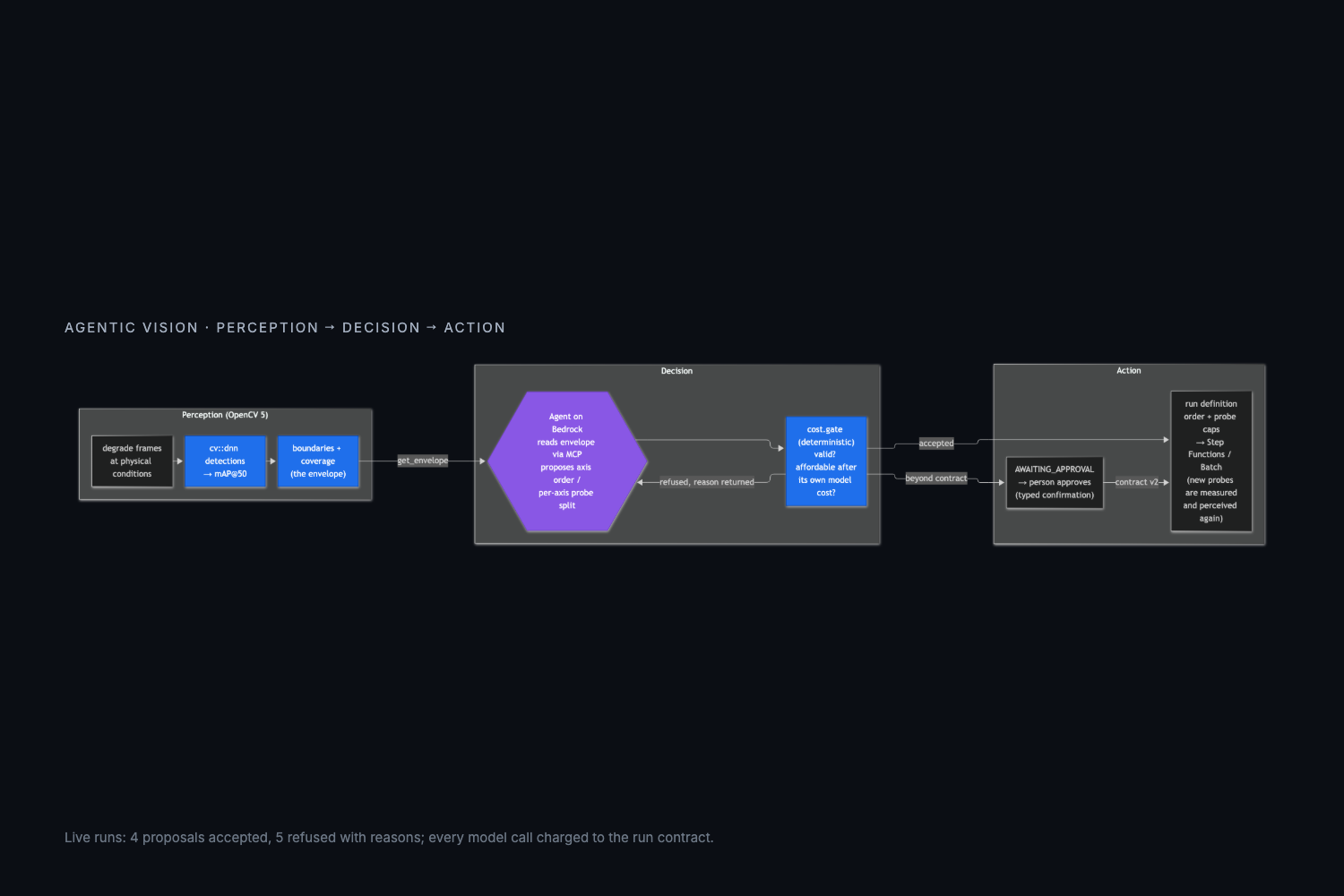
Agent proposes; deterministic gate decides; beyond-budget plans wait for a person.
-
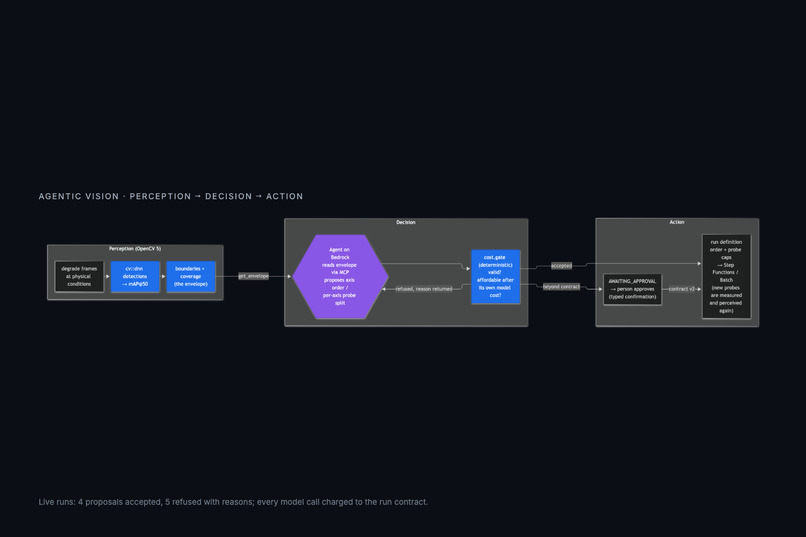
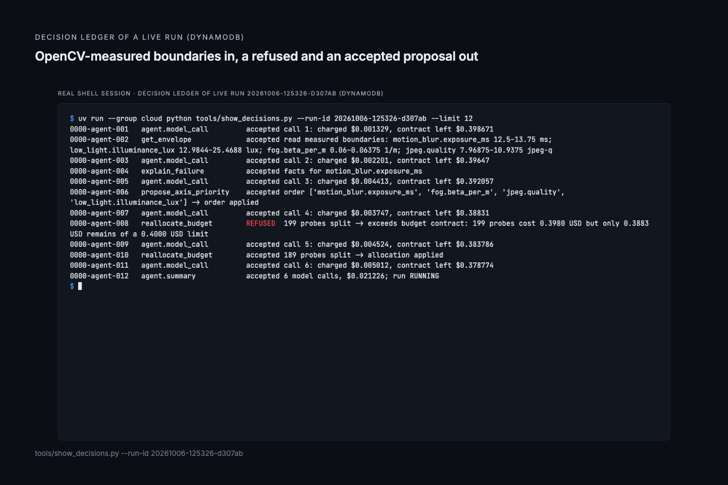
Live decision ledger: OpenCV-measured boundaries in, a refused and an accepted proposal out.
Inspiration
My day job is hardware-in-the-loop testing: we never trust a flight controller until we have pushed simulated physical conditions past the point where it breaks. Vision pipelines rarely get that treatment. A detector is usually validated on a fixed test set, and nobody can say at what exposure time or at how many lux it stops working. I wanted the same discipline for cameras: physical inputs, a measured failure boundary, and an honest list of the conditions that were never tested.
What it does
Blindspot takes a detection pipeline and a validation set, degrades the images in physical units (exposure in ms, illuminance in lux, fog extinction in 1/m, JPEG quality), and searches for the exact condition where detection fails. It reports:
- the failure boundary on each axis and across pairs of axes,
- the uncovered regions: the share of the condition space your validation set never exercised (this is the first field in every report),
- evidence frames: the wrong detections that the degradation caused, each with a command that reproduces the same number.
At 15.6 ms exposure and 173 lux, YOLOX-S reports a blurred bus as "car 0.60". The command printed under that frame reproduces the same mAP exactly.
How I built it
- OpenCV 5 for every degradation kernel: motion blur from exposure and angular velocity, defocus from aperture and subject distance, lens distortion via
remap, rolling shutter, fog from an extinction coefficient, low light with Poisson–Gaussian sensor noise, and JPEG recompression. Detectors run throughcv::dnn(YOLOX-S and NanoDet, ONNX). - Determinism first. Every kernel is a pure function of
(image, params, seed). Same seed, byte-identical output, verified across separate processes. - Boundary search instead of a grid. A verified bisection scans first and refines second, so it cannot miss a failure band in the middle of the range. A 2-D sampler maps pairs of axes.
- No LLM in the judgment path. Metrics, boundary decisions and cost limits never import an LLM client; a test checks the import graph.
- AWS, deployed with one
cdk deploy. Step Functions runs the search in rounds; each round fans out to AWS Batch on Fargate, where the same worker image runs on Graviton (arm64) or x86. Every probe writes a record to DynamoDB, and the planner is a pure function of that ledger that replays the local search, so a cloud run visits exactly the same probes. A full four-axis run on 100 frames took 14 min 41 s on Graviton, used 33 Fargate tasks and cost $0.0749 measured from billed task time, against a $0.40 per-run contract; all four boundaries were identical to the local run. Torn down and redeployed from a fresh clone by following only the README, it reproduced the same four boundaries for $0.0752. A deliberately starved contract stopped the run after four probes; it continued only afterblindspot approverecorded an approver, an amount and a reason as a new contract version. In that test the approval command was issued by my automation, not typed by a person. - Report viewer: https://d18du1w0ii5yhw.cloudfront.net/ — a static Next.js export in a private S3 bucket, served by CloudFront through origin access control. No login, no API: the page and its report JSON are plain files, so the report stays readable even when the control plane is torn down.
- COOL, measured as a third arm on EC2 (same 64-probe batch, three runs per arm, time is total work per frame). Arm 1: c7i.large, x86, stock OpenCV 5. Arm 2: Graviton4, stock OpenCV 5. Arm 3: the same Graviton4 instance with the Cloud Optimized OpenCV build (
5.1.0-dev), so arms 2 and 3 differ only in the OpenCV build. Arms 2 and 3 ran on two sizes: c8g.large (2 vCPU) and the vendor-recommended m8g.4xlarge (16 vCPU). Chip effect (arm 1 vs 2, c8g.large): 368.2 ms on x86 against 502.3 ms on Graviton4, a relative speed of 0.733; at EC2 prices Graviton also cost more per frame ($0.01113 against $0.00913 per 1,000), the opposite of the Fargate result. COOL effect (arm 2 vs 3): on c8g.large COOL ran at 0.920 of the stock wheel's speed; on m8g.4xlarge at 0.952 (97.8 against 93.1 ms). On both sizes inference was slower with COOL (0.912 and 0.905) and image measurement about equal (1.006 and 1.001); mAP was identical on 63 of 64 probes. So on this workload COOL was slower on both sizes, not faster. One trap worth stating: by the median frame COOL looked marginally faster on m8g.4xlarge (1.007); total work says otherwise, and cost follows total work. Two facts bear on the result without explaining it: the stock OpenCV 5 wheel already reports KleidiCV on Linux arm64, and the listing names image operations such as resizing, thresholding and contours, while DNN inference dominates this frame time. One workload, two instance sizes; it says nothing about those operations in isolation. - Agent, opt-in (
blindspot cloud-run --agent). Claude Haiku on Amazon Bedrock (claude-haiku-4-5) reads the envelope through Blindspot's MCP tools and may propose an axis order and a per-axis probe split. Deterministic code accepts or refuses each proposal and writes every decision, refused ones included, to DynamoDB; the agent never decides pass/fail, a boundary or a cost. Its own model calls are charged to the run's budget contract as they happen, so it cannot spend the money it is splitting. In the live run it made 4 model calls for $0.0126; its split never bound (each axis needed 8 probes), so the boundaries matched the plain run exactly and the whole run cost $0.0883. Two earlier live runs stopped inAWAITING_APPROVAL: one because the gate did not yet see the agent's own spend, one because a refused split stayed pending after a smaller one was accepted. Both were bugs in my code, now fixed and tested. One of those halted runs was later approved by a person from a terminal: the contract became version 2, the held split was applied, and the run finished with the same four boundaries. The agent's written rationale also claimed that more probes raise coverage, which is wrong (coverage is a property of the validation set); the gate bounds what it can do, so the mistake cost nothing.
Built with (read from the deployed stacks by tools/aws_services.py): OpenCV 5, Python, ONNX, Next.js, AWS CDK, AWS Batch, Amazon ECS on AWS Fargate (Graviton and x86), AWS Step Functions, AWS Lambda, Amazon DynamoDB, Amazon S3, Amazon CloudFront, Amazon ECR, Amazon VPC, Amazon CloudWatch, AWS X-Ray, AWS IAM; Cloud Optimized OpenCV (COOL) as a benchmarked arm on EC2.
Challenges I ran into
- Severity direction. Low light and low JPEG quality get worse as the number goes down. My first sweep reported "no boundary" on those axes. It was my bug, not a robust detector. Search now runs in a normalized severity coordinate so the direction cannot be wrong.
- Pure bisection misses interior failure bands, because both endpoints pass. The verified mode scans before it refines; the cheap mode's blind spot is pinned by a test.
- I refused to fake an axis. The OpenCV 5 wheel exposes no rate control for H.264, so CRF 1, 23 and 45 produced identical files. Labeling another knob "CRF" would be a fake unit, so H.264 is not implemented and the evidence is documented.
- Evidence-frame honesty. My first picker showed a wrong box that existed even without degradation. It now counts only errors the degradation caused.
Accomplishments that I'm proud of
- Baseline mAP@50 on the clean set: 0.611 (YOLOX-S, 984 objects).
- Every axis has a sharp boundary: motion blur 12.50–13.75 ms, low light 12.98–25.47 lux, fog 0.0600–0.0638 1/m (about 62 m visibility), JPEG quality 7.97–10.94.
- One-axis limits overstate the safe region. At 10.75 ms and 49.5 lux each axis is inside its own 1-D limit, but together mAP falls to 0.295.
- Limits depend on the model. On the same frames, NanoDet fails in fog at about half the density YOLOX-S tolerates.
- Search efficiency depends on precision. At 1.25 ms precision the bisection needs 8 probes instead of 33 (4.12×); at coarse precision it saves nothing (1.00×). Across 24 searches (3 datasets × 2 models × 4 axes) every boundary matched the full grid exactly. In 2-D, 22 probes classified a 289-cell map with no errors; that map is 94% failures (273 of 289), which favors the method.
- x86 vs Graviton, same image and same 64-probe batch (2 vCPU Fargate tasks, three runs per side; time is total work per frame, the mean, since a few expensive conditions skew the median). x86 was faster: 443.4 ms per frame against 507.8 ms on Graviton4. Priced per frame, Graviton was cheaper: $0.01114 against $0.01216 per 1,000 frames. The OpenCV image-measurement stage was faster on Graviton (15.7 vs 20.9 ms); the gap is DNN inference, which dominates frame time. Fargate x86 is not one CPU: the three x86 tasks landed on two generations, 584.8 ms on Cascade Lake against 397.8 and 443.4 ms on Sapphire Rapids. 59 of 64 probes gave identical mAP; the rest differed by at most 0.000246.
- Sim-to-real: the low-light model is too pessimistic. No first-party capture was made; the real photos come from the NOD night-photo dataset (Morawski, Chen, Lin, Hsu, BMVC 2021; https://github.com/igor-morawski/NOD), images licensed
CC BY-NC-SA 2.0, used here as a non-commercial research benchmark: aggregate metrics only, no NOD image or derived image is published. On 286 night photos with 668 labelled cars, even the darkest fifth (estimated median 1.08 lux) kept mAP@50 at 0.400, above the failure threshold of 0.367. At the same estimated light and the cameras' recorded exposure time, Blindspot's synthetic model predicted 0.00021. Real and synthetic agreed on pass/fail in 1 of 5 illuminance bins; in the other 4 the synthetic model predicted a failure that did not happen. The real failure point was never reached, so the gap is a bound: the synthetic boundary (12.98–25.47 lux) overstates the failure illuminance for these cameras by at least 12.0×. Illuminance is estimated, not measured: the exposure time, aperture and ISO the cameras recorded, put through the incident-light exposure equation and scaled by each photo's brightness. One plausible reason, not tested: real cameras raise gain and denoise in-camera, which the synthetic sensor at fixed gain does not. The tool measured its own blind spot, and the error is on the conservative side: it over-warns rather than misses failures. The model is deliberately not calibrated against these photos, because calibrating and validating on the same images would be fitting to the answer. Next step: model the camera's image-signal-processor noise reduction, then validate on a separate real set.
Known limitations
- Sim-to-real is measured on third-party photos (NOD,
CC BY-NC-SA 2.0, non-commercial research use) with estimated illuminance, not a first-party capture with a light meter. The low-light model was not calibrated against them (that would fit to the answer); modelling in-camera noise reduction is the next step. It covers the low-light axis only; motion blur, fog and JPEG have no real-world comparison yet. Detection was scored against the road-scene baseline's threshold, and the real and synthetic images show different scenes. - H.264 recompression not implemented (no rate control in the OpenCV 5 wheel).
- Results are not bit-identical across CPUs. On real x86 and Graviton Fargate tasks, 18 of 33 probes matched to full precision and the rest differed by at most 0.000142 mAP. Every pass/fail decision, and so every boundary, agreed; the closest probe was 0.0058 from the threshold, but a probe nearer than the gap could flip.
- Two detectors tested; independence of the method from the model is shown on two, not proven in general.
What I learned
A speedup without a stated precision is a number without a meaning. Writing the unfavorable results next to the favorable ones (1.00× next to 4.12×) made the project more convincing, not less.
What's next for Blindspot
- Model the camera's image-signal-processor noise reduction in the low-light degradation, then validate it on a real photo set that was not used to build it.
- Real-world comparisons for the other axes: motion blur, fog and recompression.
- An H.264 axis through an encoder that exposes real rate control, so CRF is an honest unit.
- More pipeline families than COCO-trained detectors: segmentation and tracking.
Built With
- amazon-bedrock
- amazon-cloudfront
- amazon-cloudwatch
- amazon-dynamodb
- amazon-ec2
- amazon-ecr
- amazon-web-services
- aws-batch
- aws-cdk
- aws-fargate
- aws-graviton
- aws-lambda
- aws-step-functions
- aws-x-ray
- claude
- cool-cloud-optimized-opencv
- model-context-protocol
- next.js
- onnx
- opencv
- python
- typescript
- uv
- yolox

Log in or sign up for Devpost to join the conversation.