-
-
-
-
-
-
-
-
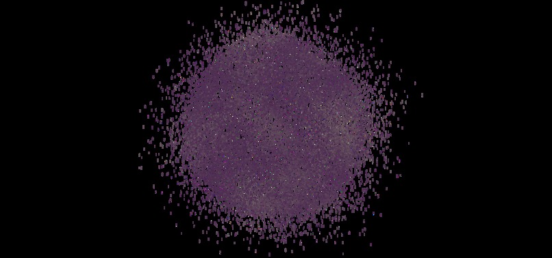
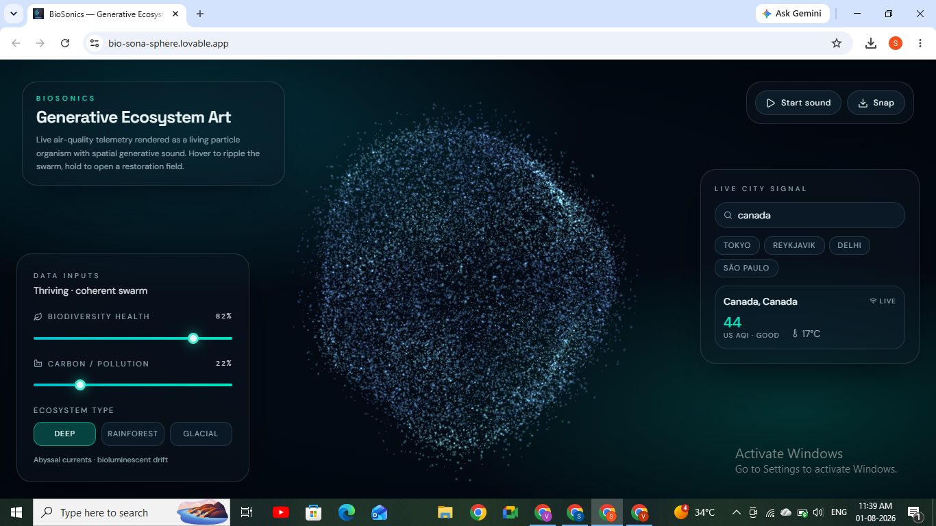
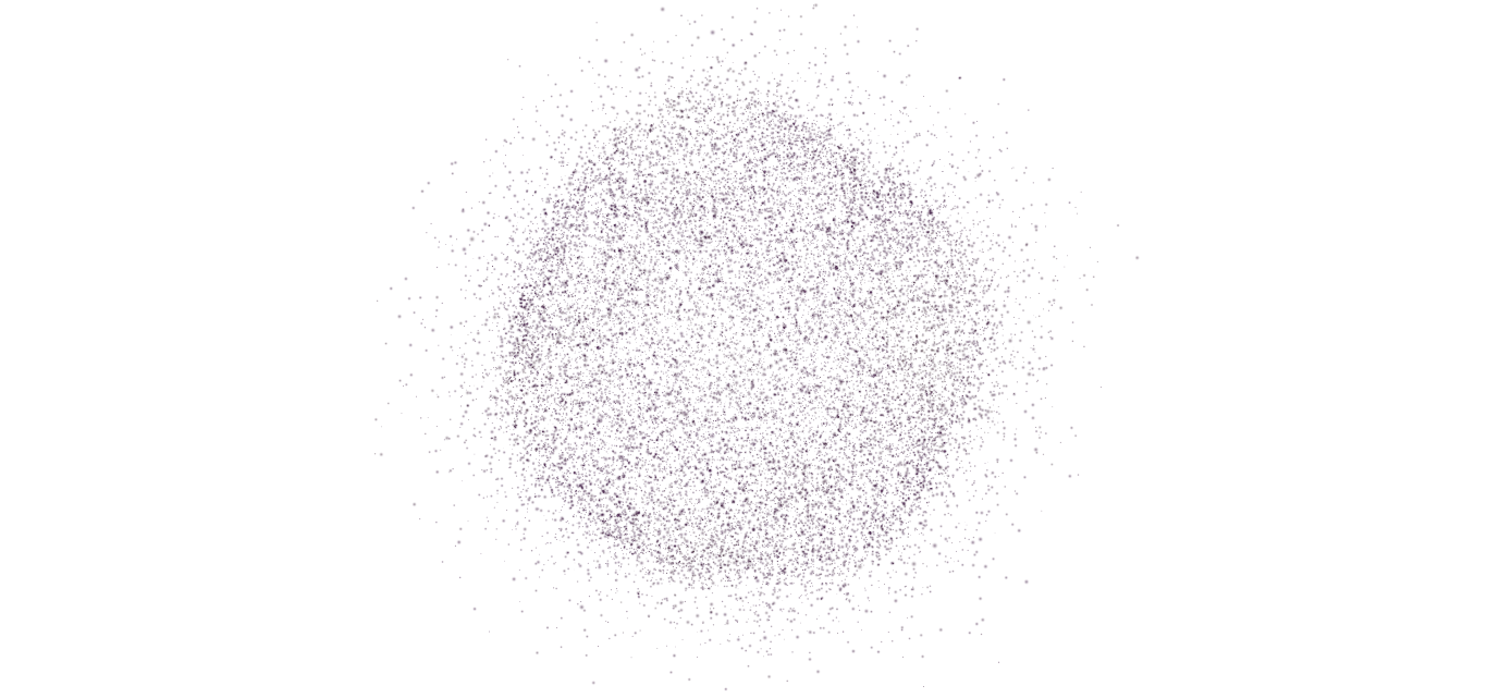
Captured Image
Inspiration
Air quality data exists as a number nobody feels. A city's AQI sits on a government dashboard, gets glanced at, and gets ignored — because a number can't make you flinch. We wanted to close that gap: take the exact same data and turn it into something with a pulse. Something that visibly struggles when the air is toxic and visibly breathes easier when it isn't.
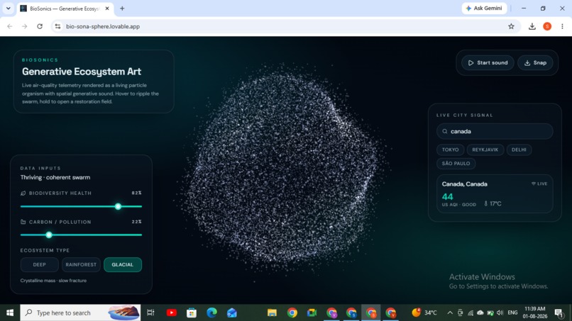
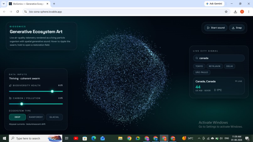
That's the core bet behind BioSonics — not "art about the environment," but art that is the environment's current state, rendered live, in three dimensions, in sound and light, generated fresh from whatever city you type in. It's not a painting of an ecosystem. It's a sculpture that only exists because a live API call fed it real numbers thirty seconds ago — which is exactly the kind of art that has no pre-digital equivalent.
What it does
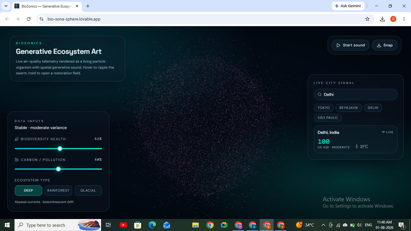
BioSonics maps a single live scalar — a city's Air Quality Index — through a chain of continuous functions into color, motion, and sound. Concretely, AQI is compressed into a normalized ecosystem health value:
$$ h = 1 - \left(\frac{\text{clamp}(\text{AQI}, 0, 400)}{400}\right)^{0.7}, \quad h \in [0, 1] $$
The exponent \(0.7\) is deliberate — it's a gamma curve, not a straight line, so moderate pollution (AQI 100–150) already produces a visibly stressed organism instead of waiting until near-collapse to react. Every other parameter in the piece — turbulence amplitude, particle color, synth dissonance, filter cutoff — is a deterministic function of \(h\), so the entire artwork is a single continuous transformation of one real-world number.
On top of that data-driven baseline, the piece is interactive:
- Search any city → geocode it, pull its live AQI and temperature, and re-sculpt the organism within seconds.
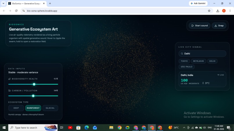
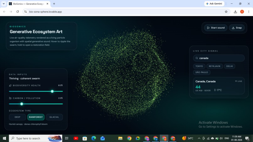
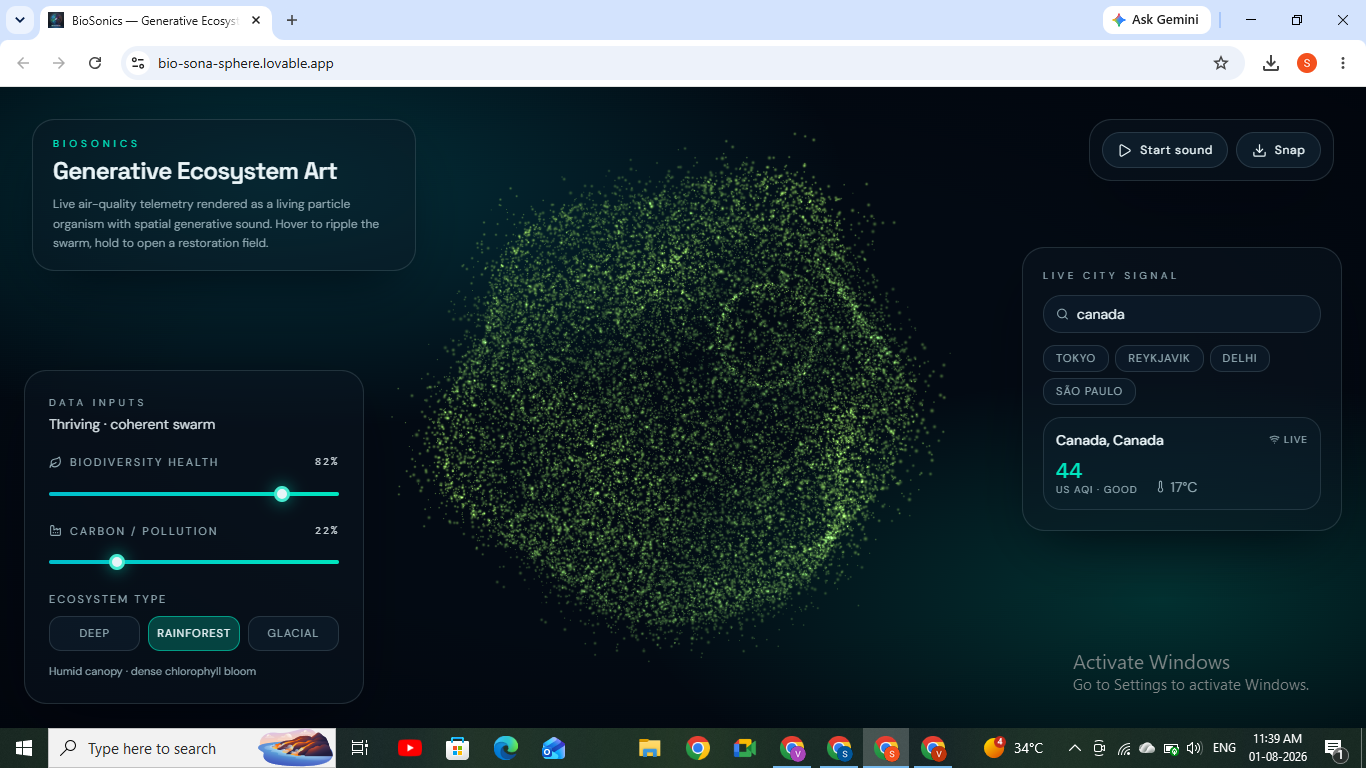
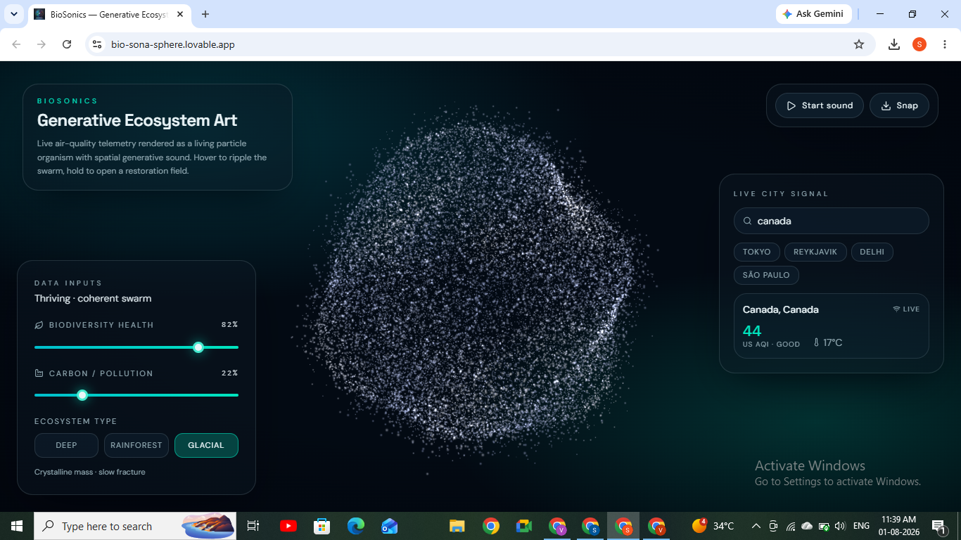
- Clean air (Reykjavik, Zurich) → the swarm resolves into a fluid, structured, emerald-and-gold form with warm, consonant harmony.
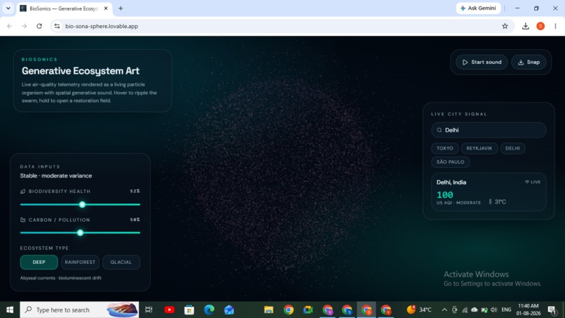
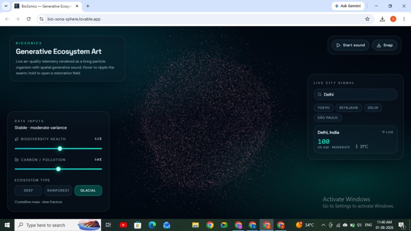
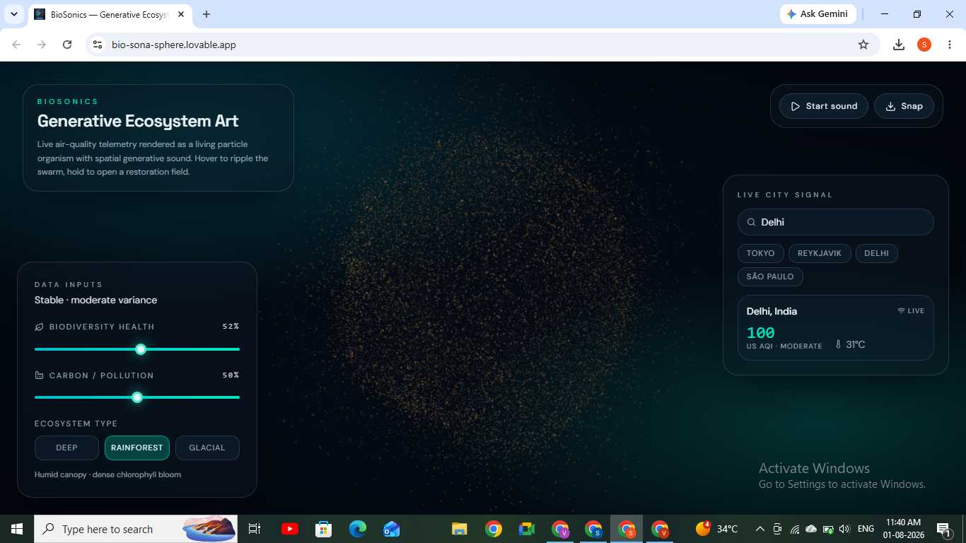
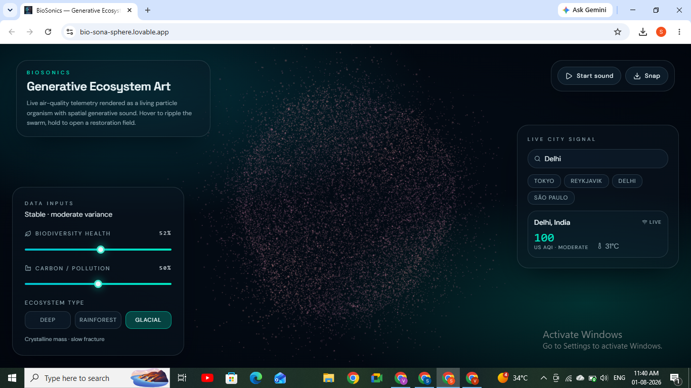
- Polluted air (Delhi, Lagos, Beijing) → the swarm fractures — dark, turbulent, flickering — while the audio degrades into filtered, dissonant noise.
- Hover → a physics-based ripple propagates across the organism's surface, sourced at your cursor's 3D position.
- Click and hold → the Restoration Field: nearby particles are pulled toward your hand, dissonance dissolves into a soothing ambient pad, and haptic pulses land in sync with the sound on supported devices.
- Snap & Export → downloads the exact artwork you generated, watermarked with city, AQI, and timestamp — every export is a unique, unrepeatable data-portrait.
No two sessions look the same. No two cities sound the same. The art is the data.
How we built it
1. Particle field — Fibonacci sphere distribution ~9,000 particles are placed on a sphere using the golden-angle spiral method, which gives near-uniform coverage without the pole-clustering of naive spherical coordinates:
$$ \theta_i = \arccos(1 - 2i/N), \qquad \phi_i = \pi(1+\sqrt{5})\, i, \qquad i = 0, \dots, N-1 $$
$$ \mathbf{p}_i = r\big(\sin\theta_i \cos\phi_i,\ \sin\theta_i \sin\phi_i,\ \cos\theta_i\big) $$
2. Organic turbulence — 3D simplex noise as a displacement field Each particle's base position \(\mathbf{p}_i\) is displaced along its own normal \(\hat{\mathbf{n}}_i = \mathbf{p}_i / |\mathbf{p}_i|\) by a simplex noise field \(\mathcal{N}: \mathbb{R}^3 \to [-1,1]\), sampled at a position that scrolls through time:
$$ \mathbf{p}_i'(t) = \mathbf{p}_i + \hat{\mathbf{n}}_i \cdot \mathcal{N}!\big(1.35\,\mathbf{p}_i + (0,0,0.18t) + s_i\big) \cdot T(h) $$
where \(s_i\) is a per-particle random phase (so particles don't move in lockstep) and \(T(h)\) is the turbulence-vs-health curve:
$$ T(h) = 0.14 + (1-h)\cdot 0.85 $$
This is the single equation that makes pollution look chaotic: as \(h \to 0\), noise amplitude nearly sextuples, and the organism visibly fragments.
3. Hover ripples — a damped traveling wave On pointer movement, a raycast gives a world-space hit point \(\mathbf{m}\). Every particle carries a radial wave sourced at \(\mathbf{m}\):
$$ R_i(t) = \sin!\big(7\,d_i - 5t\big)\, e^{-1.8\,d_i}\, \cdot S(t), \qquad d_i = |\mathbf{p}_i - \mathbf{m}| $$
where \(S(t)\) is the hover-strength envelope, an exponential decay once the pointer stops moving (\(S \leftarrow 0.94\,S\) per frame, i.e. \(S(t) = S_0 e^{-\lambda t}\) in continuous form). The \(e^{-1.8 d_i}\) term is what makes the ripple a localized pulse rather than a wave that floods the whole sphere.
4. Restoration field — a smoothstep attraction basin While the pointer is held, particles within a radius of \(\mathbf{m}\) are pulled toward it, using a Hermite smoothstep for a soft-edged basin rather than a hard cutoff:
$$ \sigma(d_i) = \text{smoothstep}(2.4,\ 0,\ d_i) = \begin{cases} 1 & d_i \le 0 \ 3u^2-2u^3, \; u=\dfrac{2.4-d_i}{2.4} & 0<d_i<2.4 \ 0 & d_i \ge 2.4 \end{cases} $$
$$ \mathbf{p}_i'' = \text{lerp}\big(\mathbf{p}_i',\ \mathbf{m}+0.22\,\hat{\mathbf{n}}_i,\ \ 0.72\,\rho\,\sigma(d_i)\big) $$
where \(\rho \in [0,1]\) is the restoration ramp — a first-order lag toward 1 while held and toward 0 on release: \(\rho_{t+1} = \rho_t + \alpha(\rho_{\text{target}} - \rho_t)\), the discrete form of \(\dot\rho = \alpha(\rho_{\text{target}}-\rho)\). This is why healing feels like an exhale rather than a switch flip.
5. Perspective-correct point sizing Rendered point size compensates for camera distance using the inverse-depth projection term, scaled by local noise and restoration for a bloom effect:
$$ \text{size}i = a_i \cdot S{\text{base}} \cdot (1 + 1.6\rho\sigma_i + 0.4|n_i|) \cdot \frac{6}{-z_{\text{view}}} $$
6. Audio — health as a continuous mixing coefficient Two synth voices run simultaneously; their gains are affine functions of \(h\), continuously cross-faded rather than switched:
$$ G_{\text{harmony}}(h) = 0.15 + 0.40\,h \qquad G_{\text{noise}}(h) = 0.06 + 0.34\,(1-h) $$
Restoration reshapes the noise voice's timbre in real time — bandpass cutoff and distortion wet mix both decay linearly with \(\rho\):
$$ f_c(\rho) = 900 - 650\,\rho \text{ Hz} \qquad w_{\text{dist}}(\rho) = 0.35(1-\rho) $$
7. Spatial position
A Tone.Panner3D (HRTF model) is bound to the same world coordinate \(\mathbf{m}\) driving the shader, so the perceived sound source and the visual disturbance point are, by construction, the same 3D coordinate — not a separate stereo-pan approximation.
Every one of these seven functions is a pure transform of either \(h\) (from AQI) or \(\mathbf{m}\) (from the pointer) — the entire piece is, mathematically, one small system of coupled continuous functions driven by two live inputs.
Data layer — Open-Meteo. Live geocoding, air-quality, and weather APIs, free and keyless, feed \(h\). A built-in offline dataset and simulated-reading fallback guarantee the experience never breaks mid-demo, even with no network.
Zero build step. Everything — shaders, audio graph, UI, data fetching — lives in one HTML file, loaded entirely from CDN. Open it and it runs; deploy it by copying it.
Challenges we ran into
The hardest problem wasn't rendering particles — it was making one number, \(h\), drive many convincingly organic parameters at once without it feeling like a slider. Turbulence, color, fragmentation, and harmonic dissonance all had to move together believably, so a lot of iteration went into tuning the easing constants (like the \(0.02\)–\(0.045\) lag coefficients on \(h\) and \(\rho\)) so the organism settles into a new state like a living thing, not a snap transition.
The Restoration Field was the single biggest rework. Our first version just faded the whole scene toward gold on click — a global lerp on color, no spatial term at all — which read as a filter, not a healing. It only became convincing once we introduced the \(\sigma(d_i)\) smoothstep basin, making the attraction genuinely local: restoration spreads outward from your actual cursor position through the swarm, matched by the noise filter and reverb opening up underneath it in the same frame.
We also had to design around the Web Audio autoplay policy — no sound can start without a real user gesture — so instead of treating that as a limitation, we made "Activate Soundscape" a deliberate, clearly-labeled first interaction that primes the audience for what's coming.
Accomplishments that we're proud of
- A shader-driven organism that stays smooth and reactive across ~9,000 live-deforming points, running the full noise/ripple/restoration math per-vertex on the GPU inside a single custom material.
- Audio that is actually spatial — position-bound
Panner3D, not a stereo-pan approximation — synced frame-by-frame to the same coordinate \(\mathbf{m}\) driving the visuals. - A restoration interaction that people intuitively understand without instructions: hold your cursor still, and you visibly, audibly, physically feel a polluted place get better.
- A genuinely small, legible mathematical core — one health value, one pointer position, and seven pure functions — producing an experience that reads as much richer than its underlying model.
- Zero dependencies, zero build tooling, one file — proof that ambitious generative art doesn't need a framework stack to feel premium.
What we learned
That a single custom GLSL shader, built around noise fields and distance functions instead of swapped materials or animation states, can carry an enormous amount of expressive range — turbulence, glow, fragmentation, and clustering all came from the same shader, just different uniform inputs and coefficients. We also learned how much a well-chosen nonlinearity matters: swapping the health curve from linear to a \(0.7\)-gamma curve alone made moderate pollution readings feel far more alive. And spatial audio turned out to be one of the most underused tools in interactive art — the moment sound started tracking \(\mathbf{m}\) in 3D, the whole piece stopped feeling like "a visualization with music" and started feeling like one reactive object.
What's next for BioSonics: Generative Ecosystem Art
- Biodiversity layer — species-loss and habitat indices layered in as a second sculptural axis, coupled into the same displacement function alongside \(T(h)\).
- Shared restoration — multiplayer healing via WebSockets, so a room full of people can restore the same city's ecosystem together, each contributing their own \(\mathbf{m}_i\) and \(\rho_i\) to a combined field.
- Time-lapse mode — replay a city's AQI history as an evolving organism across days, months, or years, animating \(h(t)\) directly from historical data.
- Sensor input — pull from real-time personal air-quality sensors (e.g. PurpleAir) so the organism reacts to the room you're standing in, not just a city you typed.

Log in or sign up for Devpost to join the conversation.