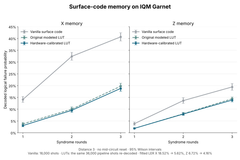
1 garnet vanilla vs calibrated lut
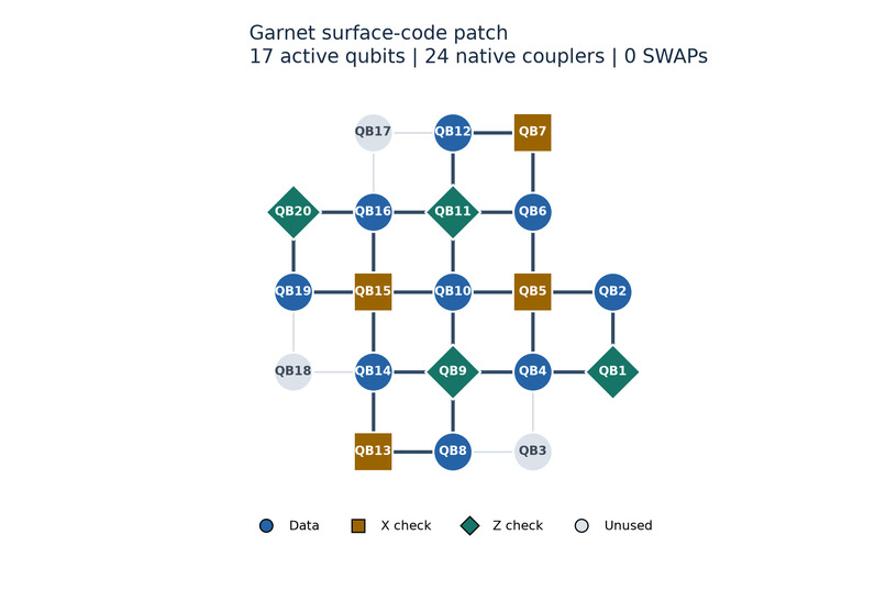
17-qubit Garnet patch on 24 native couplers, 0 SWAPs
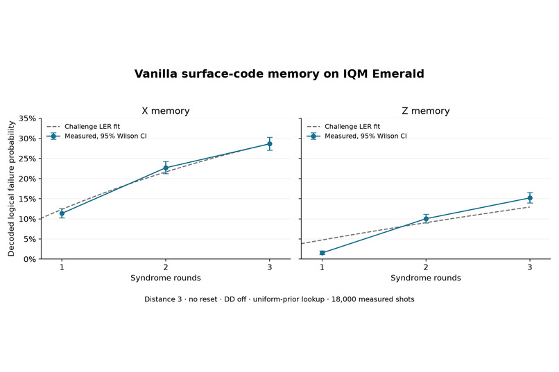
Emerald vanilla baseline with the challenge LER fit
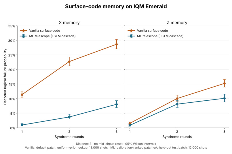
Emerald, vanilla vs ML telescope

Inspiration

The challenge asks for a surface-code memory on IQM hardware, an offline decoder and a fitted logical error rate. We wanted that number to hold up: every returned shot scored, training and test shots kept apart, and every result replayable from saved records.

We also wanted to look one step past the brief. Our best three-round Z decoder is a 16 MiB lookup table, and the table doubles with every detector bit. Twenty rounds means 160 detector bits. A machine that runs for thousands of rounds can't decode that way, so we also built a learned decoder whose size doesn't grow with the history.

What we built

A distance-3 rotated surface-code memory, run on two IQM machines.

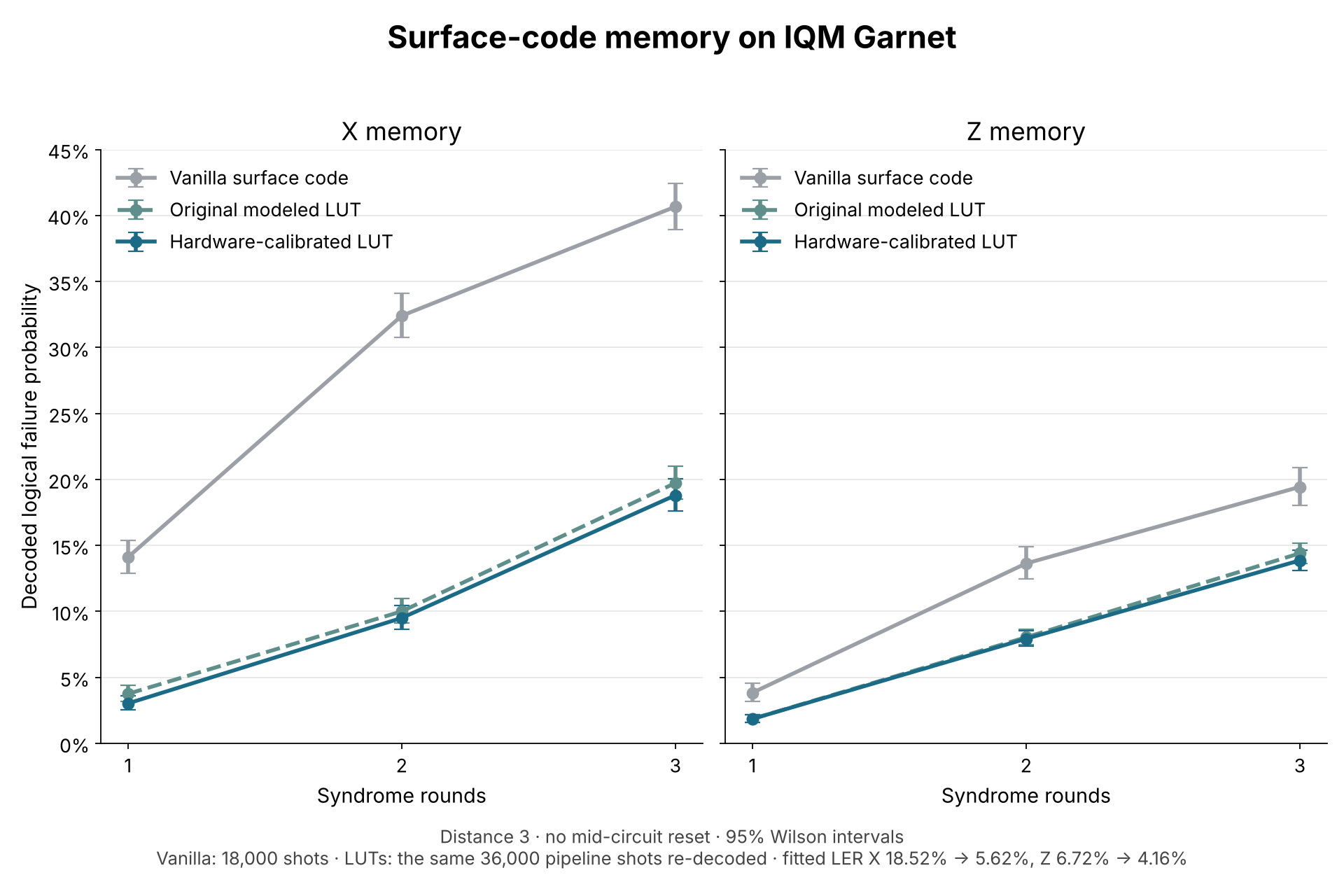
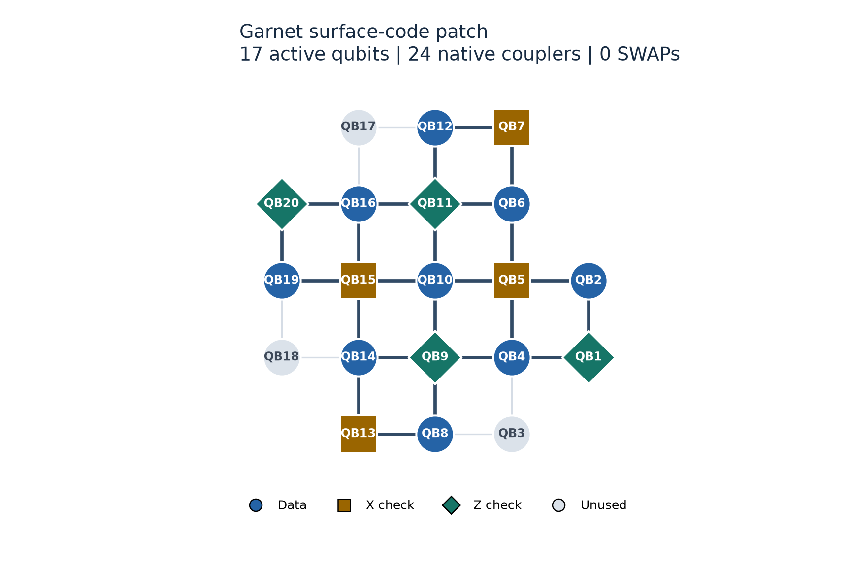
On Garnet (20 qubits) we built the full pipeline and measured it against our own vanilla baseline on 54,000 hardware shots. Fitted logical error rate (LER) fell 68.6% in X memory and 36.7% in Z memory, with the same 17 qubits, 24 CZ gates per round and zero routing SWAPs.
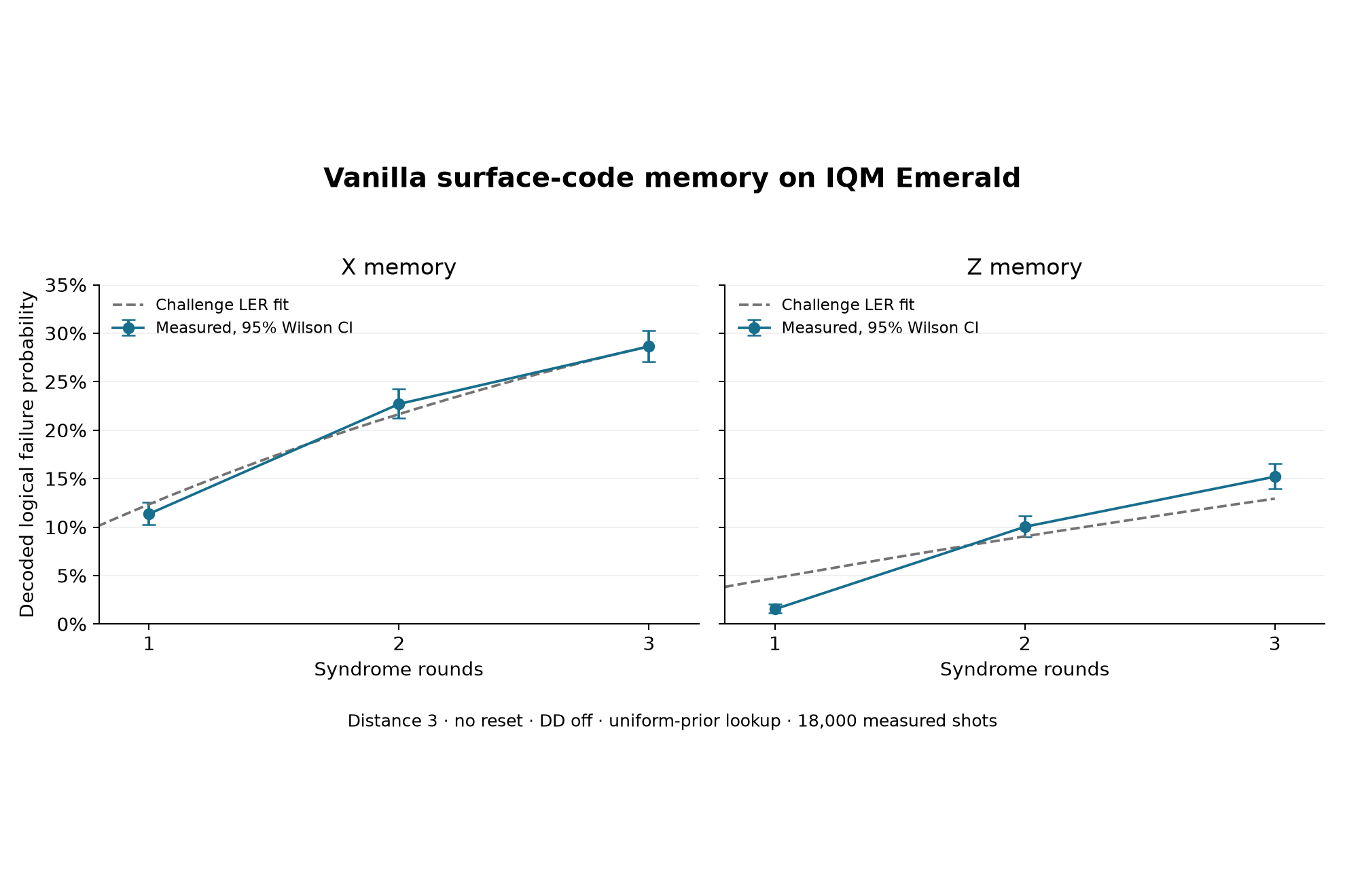
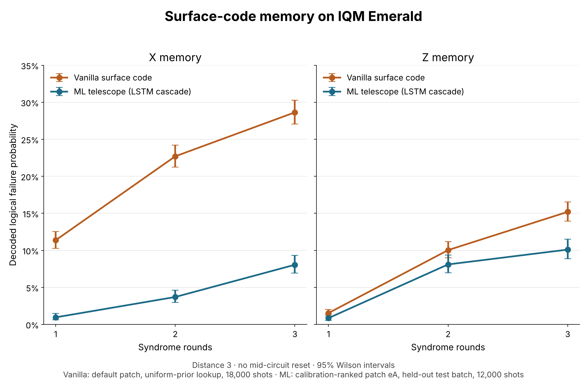
On Emerald (54 qubits) we ran an 18,000-shot vanilla baseline and an ML decoding pipeline built around a two-layer LSTM. Fitted LER fell 82.4% in X and 30.1% in Z.

Background

The code stores one logical qubit in 9 data qubits. Eight ancillas measure four X checks and four Z checks. Four weight-4 and four weight-2 checks take $4 \cdot 4 + 4 \cdot 2 = 24$ CZ gates per round. Z memory prepares logical $|0\rangle$ and asks whether bit flips get caught. X memory prepares logical $|+\rangle$ and asks the same about phase flips.

The CZ order matters. One fault on an ancilla can spread to two data qubits (a hook error). We order the four layers so each hook error lies across the logical operator of the same type, not along it, which keeps the distance at 3.

We run without mid-circuit reset, which Emerald doesn't support, so ancillas are reused as they are. Each readout $m_t$ carries the running parity, so the check value is $s_t = m_t \oplus m_{t-1}$ and a detection event compares two check values:

$$ d_t = s_t \oplus s_{t-1} = m_t \oplus m_{t-2} $$

Bulk detectors compare readouts two rounds apart. The first round, the second round and the final data readout need their own equations, so we generate them in Stim and use its measurement-to-detector converter instead of writing them by hand.

One run gives the failure probability after $r$ rounds, not a rate. We run 1, 2 and 3 rounds and fit the challenge's model by binomial maximum likelihood:

$$ P_L(r) = \frac{1 - (1 - 2\varepsilon_L)^r}{2} $$

How we built it

Circuits. A Stim generator takes distance, rounds, basis (X or Z), reset mode and an optional noise model. It writes the check schedule, the no-reset detectors and the logical observable. Each CX becomes H-CZ-H for IQM's native gate set.

Placement with zero SWAPs. We enumerate every injective embedding of the code's 17-qubit interaction graph into Garnet's coupling graph (20 qubits, 30 couplers) and rank them by summed $-\log$ gate and readout fidelity. All 24 required interactions land on native couplers. Counting SWAP instructions isn't proof, since a compiler can rewrite a SWAP as CZs and rotations. Our audit reads the compiled circuits instead: exactly $24r$ CZs for $r$ rounds, the same edge multiplicities and per-wire interaction order as the source, and routing set to none. It passes on all 12 published circuits and rejects planted SWAPs in negative tests. A SWAP count can't go below zero, so zero is optimal for this schedule.

Native compilation. We cancel redundant single-qubit rotations and schedule gates as early as their dependencies allow. Then X and Z split. In X memory the final basis rotations commute with readout on other wires, so we move them ahead of the last measurement group. The final ancilla and data readouts then form one terminal group, which IQM's compiler implements with its terminal fidelity readout. In Z memory we keep barriers between unitary and readout regions and drop only the trailing one, so the terminal readout pass still applies.

Pulse level. The optimized jobs are compiled and submitted through PulLA, IQM's pulse-level stack. Data qubits idle while ancillas are read out, so we insert XY4 (YXYX) on the 9 data qubits in those waits and audit the compiled schedule before and after. That adds 0, 72 and 144 pulse instructions at 1, 2 and 3 rounds.

A prior from the executed circuit. The decoder's noise model is built on the compiled native circuit, not the abstract one. Calibration supplies gate errors (average infidelity $e$ becomes $p = 1.5e$ for one-qubit gates and $1.25e$ for CZ) and readout error $1 - F$ for the readout type actually compiled. X memory also gets an ancilla disturbance term after each mid-circuit readout, built from IQM's repeated-readout QND and leakage metrics.

Decoders. X uses correlated minimum-weight perfect matching (PyMatching) on that prior. Z uses exact logical-class inference: a Walsh-Hadamard transform convolves every fault in the detector error model into $P(s, L)$ for each detector history $s$ and logical flip $L$. We then pull that model toward measured counts from 6,000 training shots per round count:

$$ \hat{q}(s) = \frac{k_s + 10 \cdot q_{\text{model}}(s)}{n_s + 10} $$

Here $n_s$ counts training appearances of history $s$ and $k_s$ counts the ones with a logical flip. Common histories follow the data. Rare and unseen ones follow the model. For Z we also refit fault probabilities from pairwise detector correlations, the method from Google's 2021 cyclic error correction paper, and kept the refit only where it beat the plain prior on a held-out half of the training shots. It won at 1 and 2 rounds, not at 3.

The ML telescope. A two-layer LSTM (243,714 parameters, about 488 KiB of weights) reads each round's detection events, a mask of which detectors exist that round, and the round type. It then combines its state with the final data readout to predict the logical flip. The same weights decode 1 to 20 rounds. We pre-trained on a synthetic mix built from calibration data (asymmetric readout, idling through the readout window, QND flips, leakage) and fine-tuned on hardware: 35,200 Emerald shots per basis, plus 8,800 for validation. Shots where the LSTM is unsure, $|2p - 1| < \tau$, go to Relay-BP. If Relay-BP doesn't converge, correlated MWPM decides. We chose $\tau$ on validation with a one-standard-error rule before opening the test batch. Emerald X uses $\tau = 0.19$ and sends 23% of test shots to Relay-BP. Emerald Z uses $\tau = 0$.

On Emerald we also chose the patch differently: we simulated every zero-SWAP placement under calibrated noise and took the one with the lowest predicted three-round failure.

Results

Garnet: vanilla vs our pipeline

Our vanilla baseline is already a correct memory: native zero-SWAP placement, literal H-CZ-H compilation, no DD, and a full-history maximum-likelihood lookup with a uniform $p = 0.003$ prior. Both arms ran under the same calibration, 18,000 vanilla shots and 36,000 pipeline shots.

X memory: 18.517% (95% CI 17.748 to 19.314%) down to 5.808% (5.492 to 6.136%), 68.6% lower.
Z memory: 6.722% (6.326 to 7.135%) down to 4.255% (4.066 to 4.449%), 36.7% lower.
At 3 rounds the failure probability fell from 40.67% to 18.20% (X) and from 19.43% to 14.34% (Z).
A 20,000-resample bootstrap, stratified by round and acquisition block, puts the absolute drop at 11.8 to 13.7 points for X and 2.0 to 3.0 points for Z (97.5% intervals, Bonferroni over the two bases).

Emerald: vanilla vs ML telescope

X: 12.352% (11.773 to 12.953%) down to 2.179% (1.921 to 2.459%), 82.4% lower.
Z: 4.749% (4.424 to 5.089%) down to 3.318% (2.994 to 3.665%), 30.1% lower.
At 3 rounds: X 28.63% to 8.05%, Z 15.20% to 10.10%. Vanilla used 3,000 shots per point. The ML numbers come from a separate test batch of 2,000 shots per point that never touched training or the choice of $\tau$.

Decoding time

One CPU thread (Ryzen 9 8945HS), one shot at a time. At 20 rounds the LSTM takes 38.2 µs per round on X and 39.9 µs on Z. The full X telescope takes 710 µs per round, because unsure shots also run Relay-BP, and its p99 for a 20-round history is 47.7 ms.

What we discovered

The calibration model underestimates the device, and the excess sits in the middle rounds. In a 1,000-shot Garnet pilot (Z memory, 3 rounds), correlated MWPM failed 20.9% of shots against 9.5% predicted from calibration. First-round detectors fired at 0.079 on hardware and 0.079 in simulation. Final-layer detectors fired at 0.146 and 0.145. Rounds two and three, the ones that inherit an ancilla from a mid-circuit readout, fired at 0.267 and 0.284 against 0.201 and 0.222. Detector pairs one round apart fired together at 0.063 against 0.033, which is what an ancilla flipped by its own readout looks like when there is no reset. Only adding readout-induced leakage brought the simulator close (0.061). That set the LSTM's pre-training mix, and it is why we fine-tune on real shots.

It also explains the poor constant-rate fits. Every Garnet fit has deviance far above the 5.99 cutoff for 2 degrees of freedom (52 to 199). With one round there is no mid-circuit readout at all, since the ancillas are read with the data in the final layer, so round one is cheaper than every later round. Emerald Z vanilla goes 1.5%, 10.0%, 15.2% over rounds 1 to 3. We report the fitted LER because the challenge asks for it, with the raw failure probabilities next to it.

On Emerald, most of the gain comes before the neural network. On the same test shots, correlated MWPM with our calibrated prior already fails 8.75% at 3 rounds, against 28.63% for vanilla on the default patch. The LSTM cascade takes that to 8.05%. Paired on identical shots over 1 to 20 rounds, the fine-tuned LSTM's fitted LER is 0.911 times correlated MWPM's for X (95% CI 0.881 to 0.944) and 0.964 times for Z (0.931 to 0.996).

Synthetic pre-training was enough for X but not for Z. Before fine-tuning, the LSTM already beat correlated MWPM on X (0.925, CI 0.892 to 0.959) but only tied on Z (0.998, CI 0.967 to 1.028). Hardware fine-tuning moved Z to 0.964.

Relay-BP matched matching but cost far more. On the same test shots its fitted LER was 0.997 times correlated MWPM's on X and 0.993 times on Z, at 50 to 200 times the cost per shot in our simulated benchmarks. So it only sees the shots the LSTM is unsure about.

Challenges we ran into

Bookkeeping. Sparse Stim qubit IDs, dense circuit indices and physical QB names are three separate index spaces, Qiskit reverses bit order, and native optimization reorders measurements. We store an explicit column permutation and check that the source circuit and the compiled circuit give identical detection events and logical flips on every recorded shot. A bookkeeping bug can look exactly like a physics improvement, so the replay runs this check on all 54,000 Garnet shots.
The lookup table. Full-history tables take 256 B, 64 KiB and 16 MiB at 1, 2 and 3 rounds, and building the last one needs a 512 MiB transform. At $2^{8r}$ entries, 4 rounds would need 4 GiB and 20 rounds $2^{160}$ entries. That pushed us to the LSTM.
Relay-BP wasn't deterministic. The package redrew its random memory strengths on every call, so about 0.5% of decisions depended on which shots were decoded earlier in the batch. We draw them once per decoder from a seeded generator and pass them in. Its Rust build also failed on one of our machines.

How this maps to the judging criteria

Correctness (30%): generated no-reset detectors, a source/native frame check on every shot, offline replay of all hardware data.
Sophistication and SWAPs (30%): zero routing SWAPs with an audited certificate, exactly $24r$ CZs, calibration-ranked placement, readout fusion and fences, pulse-level XY4.
LER statistics (20%): binomial maximum-likelihood fits with profile intervals, Wilson intervals per point, a stratified bootstrap for the comparison, and deviance reported where the model fits badly.
Flexibility and advanced features (20%): two QPUs, both memory bases, pulse-level DD, calibration-built priors, correlation fitting, and an LSTM with Relay-BP and MWPM behind it.

Reproduce it

From the repo root with Python 3.11+, run python -m pip install -e ".[test]" -e ./ethan. Then:

python -m examples.reproduce rebuilds detector frames for all 54,000 Garnet shots, decodes them, and refits both LERs and the bootstrap. It runs offline.
python -m challenge.audit_garnet_routing checks the zero-SWAP certificate.
python -m examples.replay_emerald replays the 18,000-shot Emerald baseline.
python -m MLfolders.mlDecoder.compare_emerald recomputes the ML comparison and per-round timings.

What's next

Put decoding in the control loop. A three-round Garnet run spends under 4 µs on everything after its 298 µs passive reset. Our LSTM needs about 38 µs per round on one CPU thread, so time per round has to become a target next to LER.
Train one recurrent model across code distances and larger patches.
Distance 5 on Emerald, and logical operations instead of memory alone.

AI tools we used: Claude Code, Claude (web), Codex, ChatGPT.