AquaGuard

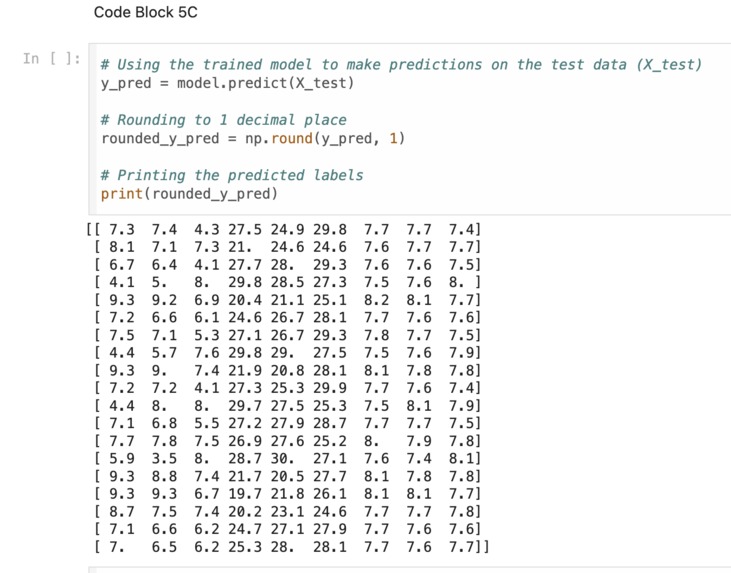
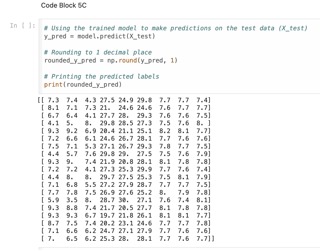
Prediction Values
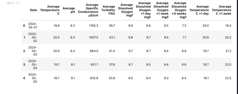
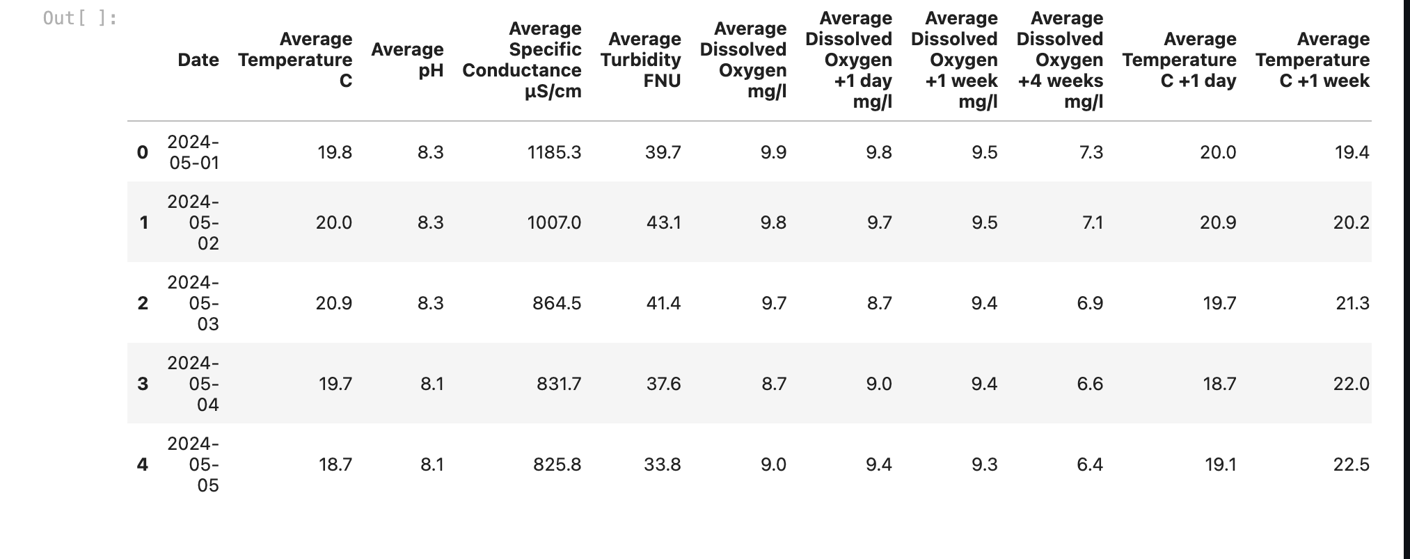
Database on Google Colab
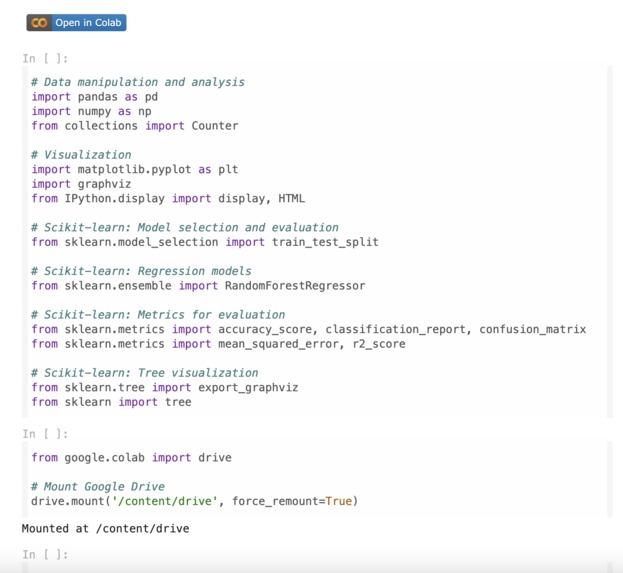
Python Libraries
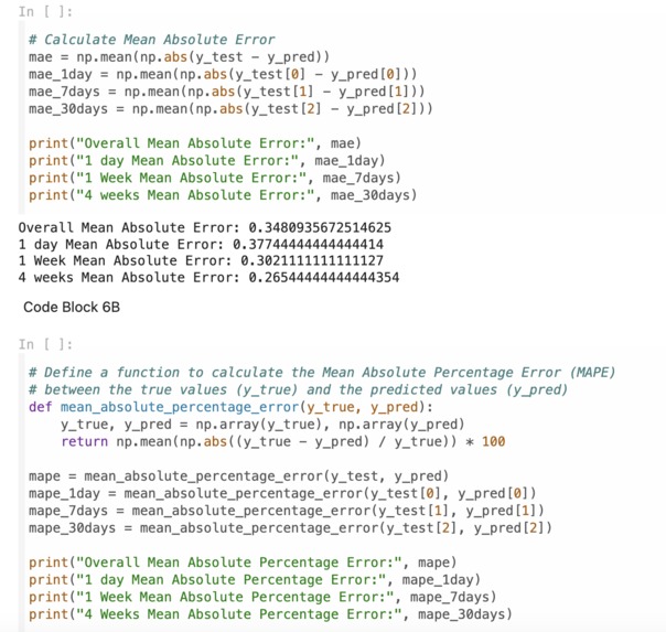
Mean Absolute Error, Mean Absolute Percent Error
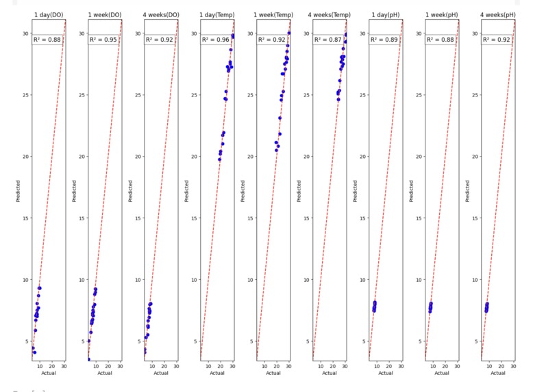
R-Squared Graphs
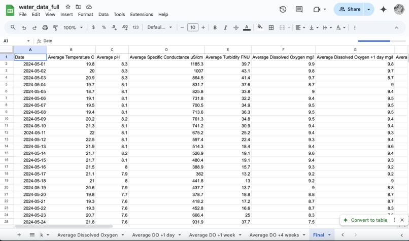
Google Sheets Database

Inspiration

     All of our team members shared a passion for marine biology and the protection of marine life. After discussing the sub-topics of this field, we concluded and combined interest in creating a project related to the prediction of water quality.

How we built it

     To begin, our team, after researching the various national water databases, selected the USGS National Water Dashboard with its consistently updated database every 15 minutes, as well as the simple exporting of the data in this database led us to select this site. 
     After securing our database, our team needed to select a local water source to collect the data from, and after thorough research, we decided to choose the San Joaquin River, as our research displayed how there have been prior studies on its water quality, and that it has displayed signs of excessive nitrates, giving us an interesting database to work with. 
    After deciding our location, further research needed to be conducted regarding which water quality indicators are the most crucial to marine ecosystems, along with their calculation metrics, as these would be the parameters we would implement in our project. Through our research, we determined that dissolved oxygen, temperature, pH, turbidity, and specific conductance were some of the most influential factors determining water quality in a body of water, and we finalized these 5 factors to be our project prediction parameters. 
     With these parameters selected, our team’s following order of business was to find a location along the San Joaquin River in one of the USGS national water stations that was available with the aforementioned parameters. After extensive searching, our team located the San Joaquin River Station in between the Newman and Merced areas, which we then located the source page of from USGS.

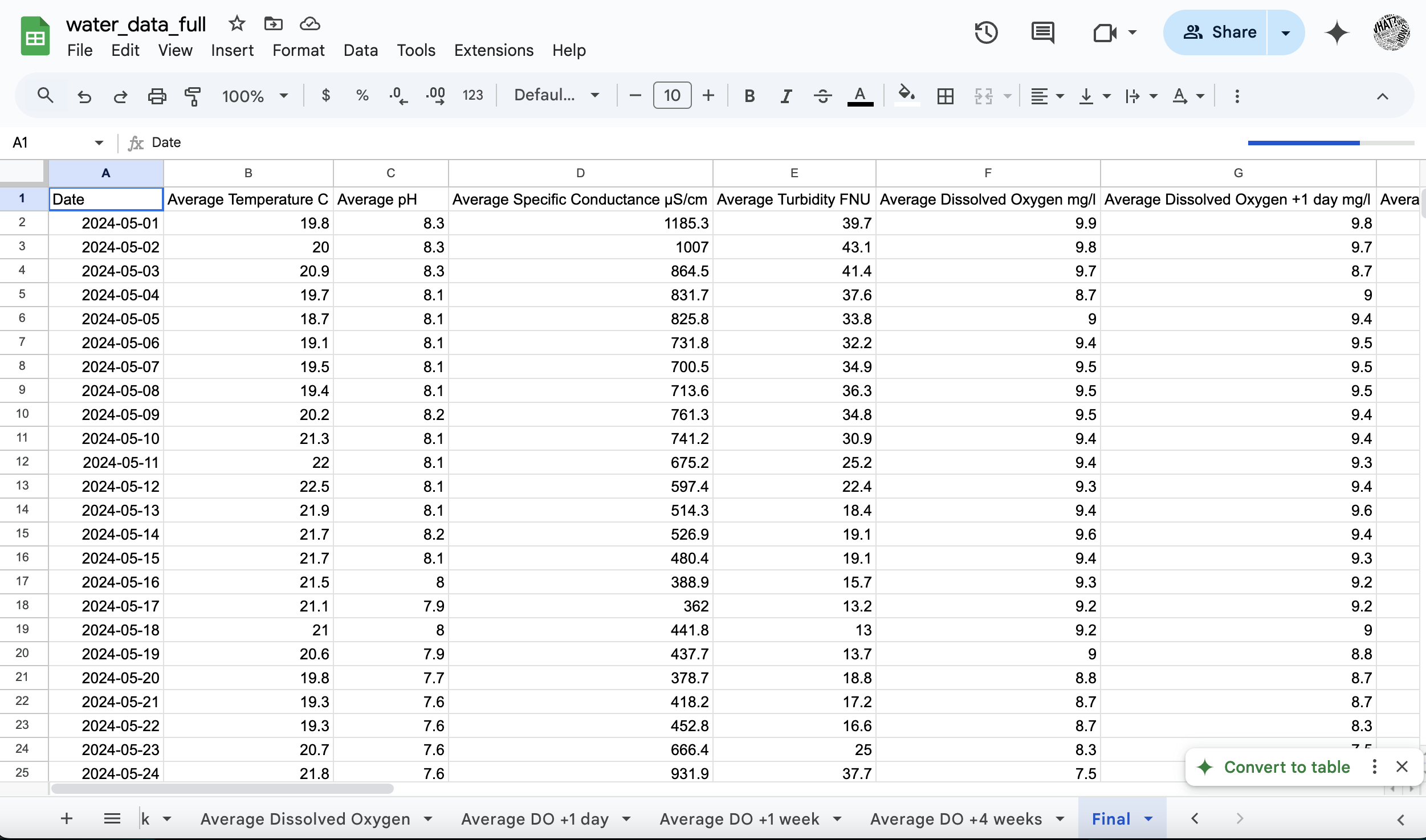
In the source page, we set our time frame between May 1, 2024, and August 1, 2024, ensuring a 3-month data span with at least one month of data following the data set. After selecting our desired time frame, we collected the “Primary Time Series” from USGS, which we copied into our Google Sheets Database, and formatted, leaving only the date, time, and value of each parameter, along with the date and average of each day. The same process was repeated for the time spans of one day, one week, and four weeks after the set data span, and for all of the 5 parameters we chose. We split the coding of the prediction value into 6 steps:

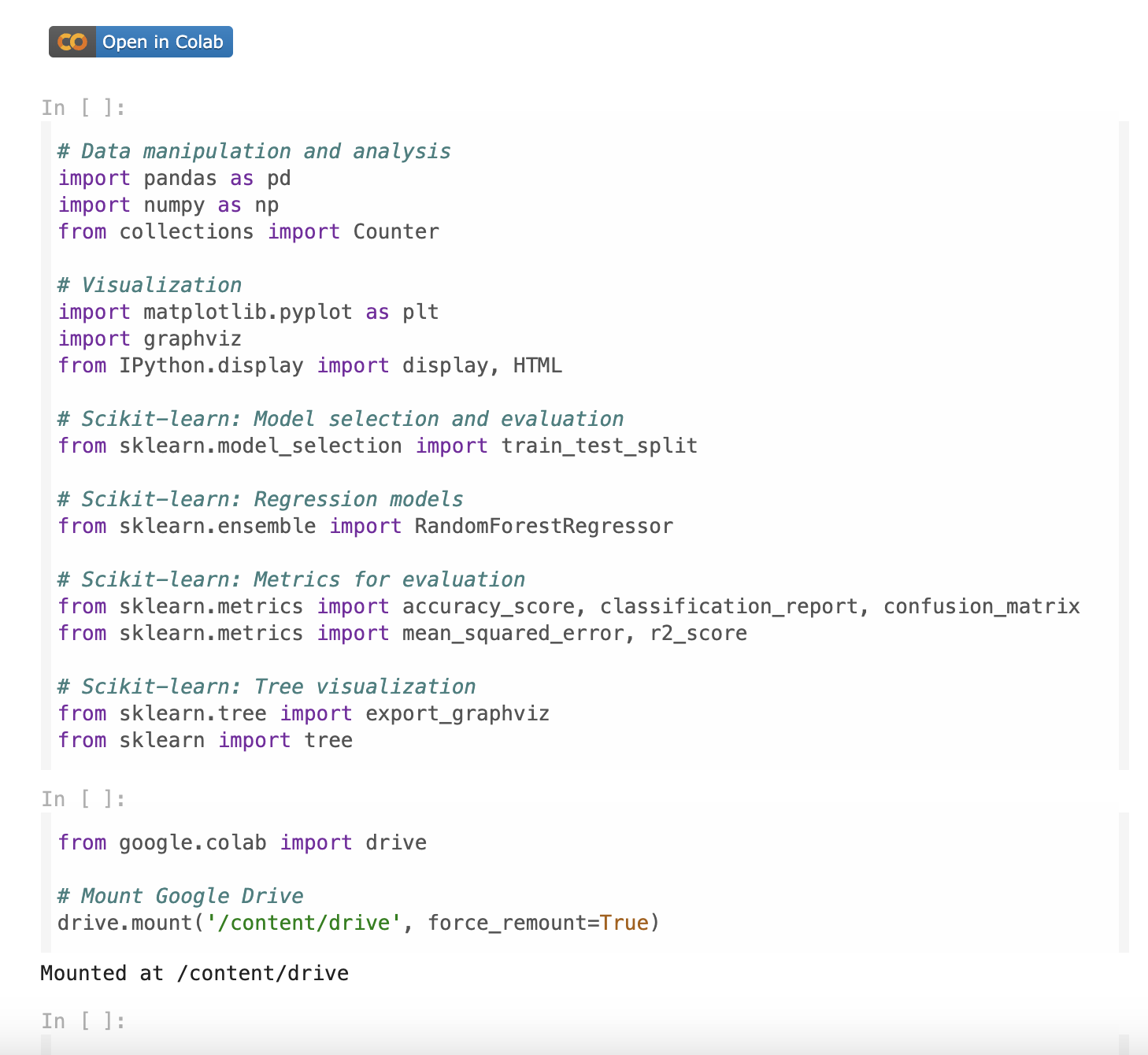
Importing libraries for Data Visualization, Data Manipulation and Analysis, Model Selection, and Model Evaluation Metrics
Connected Our Google Drive
Loaded the CSV (Comma Separated Values) File of our Google Sheets Data Base
Processing the Data Set (Selecting Target Columns, Converting Data to Float Values, Splitting the Training/Testing
Initializing the Model + Prediction Values(Rounded)
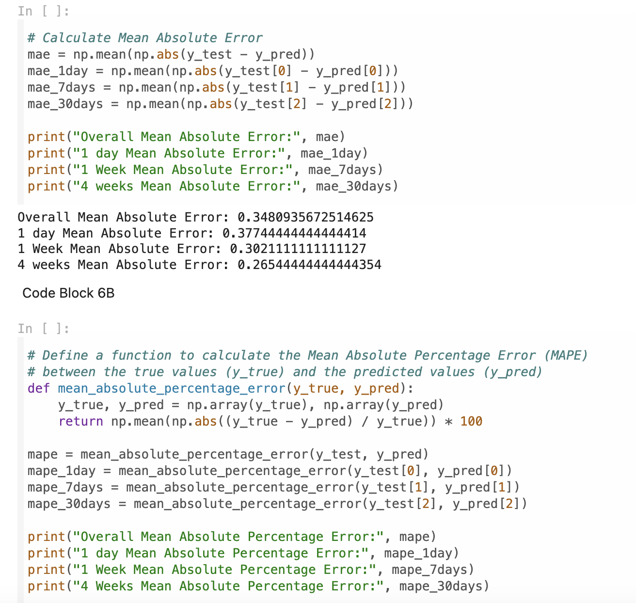
Model Evaluation (MAE and MAPE
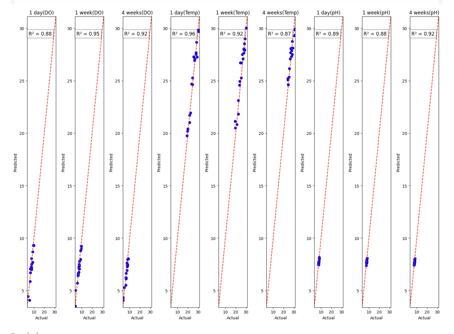
Data Visualization (Plotting the r^2 Value)

To expand: our team imported pre-existing Python libraries created by others for public use to assist our process. For Data Analysis and Manipulation, we imported Pandas and Numpy as our main libraries, abbreviated as pd and np respectively. The central library we utilized for Visualization is Matplotlib.pyplot, abbreviated as plt, and for the regression model integration, and evaluation metrics, the main libraries that we referenced to was Scikit-learn, or sklearn. Moving on to step two, this is a simple step importing our google drive from Google Colab and mounting it in the project.
For step 3, our code defines a path for the model to take in order to reach the CSV file, which is our Google Sheets Database, and then asks the model to read the file and import the data into Google Colab. In the 4th step, our team selects the target data frames needed for defining our features and predictions, along with converting the values in our databases to floats (decimals that reduce error in the code). The 4th step also splits the data from our database into a training and testing set, with training having 80% and testing having 20% of the data.
Step 5 encompasses the initializing of the Random Forest Regressor model, fitting the model to the training data, and making the predictions rounded to the nearest tenth.
The 6th step contains the model’s accuracy metrics, of Mean Absolute Error and Mean Absolute Percentage Error, using equations to calculate these values.
The seventh and final step creates the plot for graphing our R-Squared value, and displays these graphs underneath.
As for the Feature Importance aspect, the 1-5 steps remain the same, but the 6th step is the final step and creates a model estimator tree usign our features and explains the correlation between the values of the parameters, adn also codes for a bar graph explaining the importance of each feature in calculating each parameter.

Challenges we ran into

    In our project, we faced multiple challenges. To start with, we had to find a compatible and efficient platform on which to code. We were stuck on which of our numerous options would perform the best as our coding platform. We finally decided on Google Colab since it fit our requirements the best, and allowed for seamless integration between Google Sheets Database and Colab.
Next was our time span. During the hackathon, we knew we only had 24 hours to complete our ambitious project. This required us to stay focused throughout the time span, and delegate tasks efficiently. Not only did we finish, but we also had much time to spare to polish our project.
To continue, we needed an efficient way to split up the tasks between our members which ensured everyone was contributing. This was an issue for us as many of our members weren’t proficient in coding. We decided to have our members work with the parts that are related to their strengths. This way we could know that each part of the project was of the highest quality.
Finally, we encountered issues when managing Github. Since it was our first time working with the platform, it was tough learning how to use it. The same was true for git and coding on iTerm2. To combat this issue, we learned basic code through trial and error and watched tutorials to create our repository.

What we learned

During the development of our algorithm, we gained valuable lessons about teamwork, creativity, and passion. Collaboration became a key part of our journey, as each team member contributed unique strengths and perspectives. We learned the importance of clear roles, balanced workloads, and supporting one another, which strengthened our teamwork and improved our project. Creativity was equally important, pushing us to think outside the box and find innovative solutions to challenges. Passion fueled our determination, keeping us motivated through long hours and setbacks. This shared enthusiasm turned our ideas into reality and helped us create a project we were proud of.