• 

About the Project

Inspiration

Vascular anatomy is highly variable from patient to patient, yet much of surgical planning still depends on manually reviewing CT angiography slice by slice.

We were inspired by a simple question:

Can we turn a CT scan into a structured, machine-readable map of vascular anatomy?

For this challenge, we focused on the abdominal aorta. Given only a CTA volume and a binary mask of the parent aorta, our goal was to automatically discover the arteries that directly branch from it and describe each branch quantitatively.

Instead of treating medical imaging as something that can only be viewed, we wanted to treat anatomy as something that can be computed, measured, and explored.

---

What We Built

We built an end-to-end vascular branch discovery and visualization pipeline.

The user uploads:

• a 3D CTA volume
• a binary mask containing the abdominal aorta

Our system then analyzes the region surrounding the aorta and searches for candidate daughter vessels based on several properties:

• similarity to contrast-enhanced aortic blood intensity
• direct connectivity to the aortic wall
• continuity through 3D space
• tubular geometry
• sufficient vessel length beyond the ostium

For every detected direct branch, the system estimates:

• Ostium — where the vessel originates from the aorta
• Seed point — the vessel center approximately 5 mm downstream
• Direction — a unit vector describing the initial branch direction
• Radius — the local vessel radius near the seed point
• Proximal branch path — followed for up to 10 mm or until the first downstream bifurcation

The results are converted from voxel coordinates into physical millimeter coordinates and exported as structured JSON.

To make the predictions interpretable, we built two complementary visualizations:

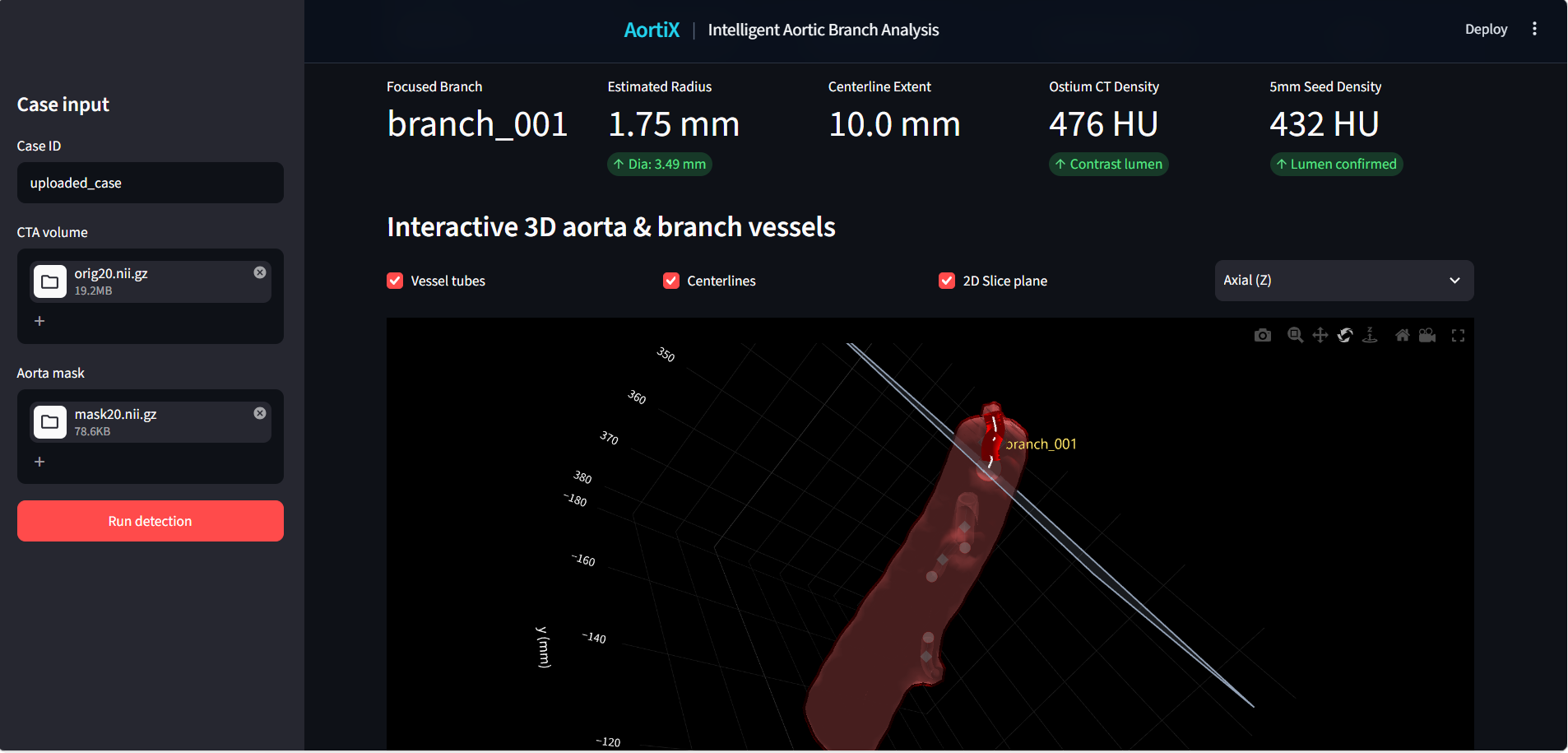
Interactive 3D View

The reconstructed aorta and detected daughter vessels are displayed in an interactive 3D environment, allowing users to inspect:

• vessel geometry
• detected branch origins
• centerlines
• branch relationships
• corresponding anatomical locations

Annotated 2D CT View

Each prediction is also mapped back onto the original CTA slices.

This allows users to verify the detected ostium, seed point, radius, and direction directly against the source medical image rather than relying only on a reconstructed 3D model.

Together, the 2D and 3D views create a bridge between raw medical imaging and machine-readable anatomical structure.

---

How We Built It

Our pipeline is centered around the provided aortic mask.

Rather than searching the entire CT volume, we first construct a local search region around the aorta. This significantly reduces the amount of data that needs to be processed.

We use SimpleITK to load the NIfTI volumes and preserve important medical imaging metadata such as:

• voxel spacing
• image origin
• image orientation
• physical coordinates

The CTA and aortic mask are converted into NumPy arrays for image processing.

We then create a physical-distance shell around the aorta using a 3D Euclidean distance transform. Candidate vessel structures within this region can then be evaluated using intensity, connectivity, and geometry.

The overall pipeline is:

CTA + Aorta Mask
        ↓
Validate image geometry
        ↓
Create local search region around the aorta
        ↓
Identify candidate vascular structures
        ↓
Find structures directly connected to the aortic wall
        ↓
Locate candidate ostia
        ↓
Trace each candidate vessel in 3D
        ↓
Reject candidates that cannot be followed for at least 5 mm
        ↓
Follow valid branches up to 10 mm or the first bifurcation
        ↓
Estimate seed, direction, and radius
        ↓
Convert voxel positions to physical millimeter coordinates
        ↓
Generate JSON + 2D + 3D visualization

Challenges We Faced

One of the biggest challenges was that a bright structure near the aorta is not necessarily a true aortic branch.

The supplied mask contains only the parent aorta, while daughter vessels are visible in the CTA but are not labelled. This means our system has to discover branch origins directly from the image using vessel appearance, 3D continuity, and connectivity to the aortic wall.

Several structures can create false positives:

• nearby veins
• calcifications
• bones and other high-intensity structures
• vessels that pass close to the aorta without actually connecting to it
• partial-volume effects that can make nearby structures appear connected

Because of this, simple intensity thresholding was not enough.

We approached branch detection as a combination of:

• intensity similarity
• 3D continuity
• tubular geometry
• direct connection to the aortic wall
• minimum vessel length

A valid daughter vessel must remain traceable for at least 5 mm beyond the aortic wall.

We measure the traced vessel path using:

$$ L = \sum_{i=1}^{n-1} \left| \mathbf{p}_{i+1} - \mathbf{p}_i \right|_2 $$

and reject candidates that cannot be followed for at least 5 mm.

Once a branch is confirmed, we continue tracing its proximal path for up to 10 mm, or until the first downstream bifurcation, whichever occurs first.

This introduces another challenge: branch geometry can change quickly after leaving the aorta. A vessel may curve immediately, split early, or pass close to another vessel, so tracing must preserve the correct daughter path without jumping to nearby structures.

We also had to handle several important anatomical edge cases:

• Two nearby origins must remain separate if they form distinct openings at the aortic wall.
• A common trunk counts as one direct aortic branch even if it bifurcates shortly afterwards.
• A vessel arising from another daughter must not be counted as a direct aortic daughter.
• The flat superior and inferior ends created by cropping must not be mistaken for branch origins.
• A nearby vessel that only touches or passes close to the aorta must not be treated as connected.

Built With

• python
• streamlit