AI Image Detection

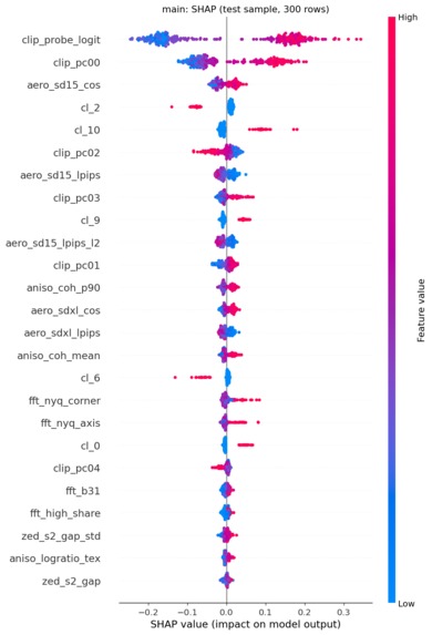
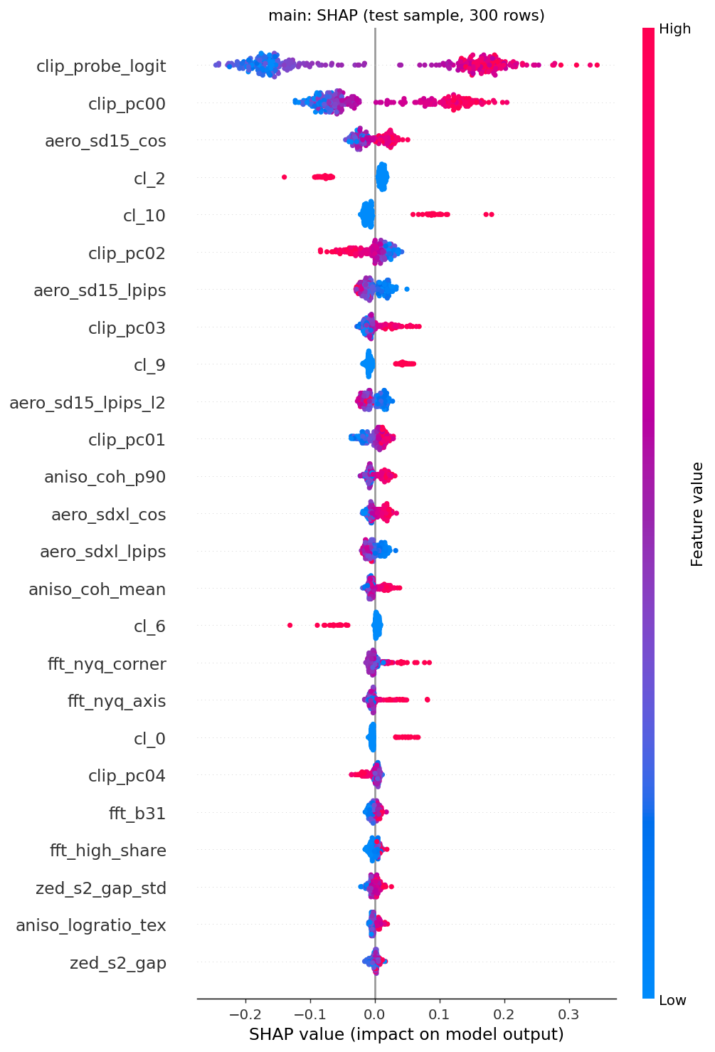
Red dots are ai, blue are real
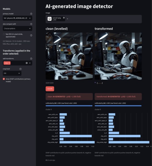
Our AI Image Detector Dashboard

Inspiration

Most AI-image detectors are black boxes: fine-tune a large network on real and fake images and it says "fake" or it doesn't. When it works nobody can say why, and when it fails on a new generator or a re-compressed screenshot nobody can say why either. In a world where the biggest black-box models get all the attention, we wanted something we could explain.

The question that drove us was: what is physically different about a generated image? A camera photo carries the fingerprints of a real sensor and a real scene — noise that grows with brightness and is independent of content, edges whose orientation agrees at every scale, colour-channel correlations left by demosaicing. A generator has none of that history and leaves its own traces instead: periodic grids from upsampling layers, latents its own decoder can reproduce almost perfectly, pixels that a compressor trained on real photos finds "too easy". Every one of those is a measurable quantity with a reason behind it. We went to the forensics literature, turned those ideas into named features, and made interpretability the design constraint rather than an afterthought.

What it does

It classifies an image as real or AI-generated and returns a calibrated probability — p(AI) = 0.8 means about 80 % of images scored that way are AI — together with an explanation of which measurements drove the verdict.

Every image is converted into ~130 named features from five families:

Physics trio (adapted multiLID) — gradient-covariance anisotropy, cross-scale orientation consistency, noise–signal decoupling, plus cross-channel residual correlation. No learned parameters.
FFT — radial power spectrum, spectral slope, band energies and the peaks upsampling layers leave at ½, ¼, ⅛ of Nyquist. No learned parameters.
AEROBLADE — reconstruction error through three latent-diffusion VAEs (SD 1.5, SDXL, FLUX.1): generated images survive an encode→decode round trip almost losslessly; photos do not.
ZED — "coding-cost surprise" from a lossless coder pre-trained on real photos: generated pixels are cheaper to encode than the coder expects.
CLIP ViT-L/14 — a semantic embedding, used as principal components, a cross-fitted linear probe, and unsupervised clusters that let the model weight features differently per image sub-type.

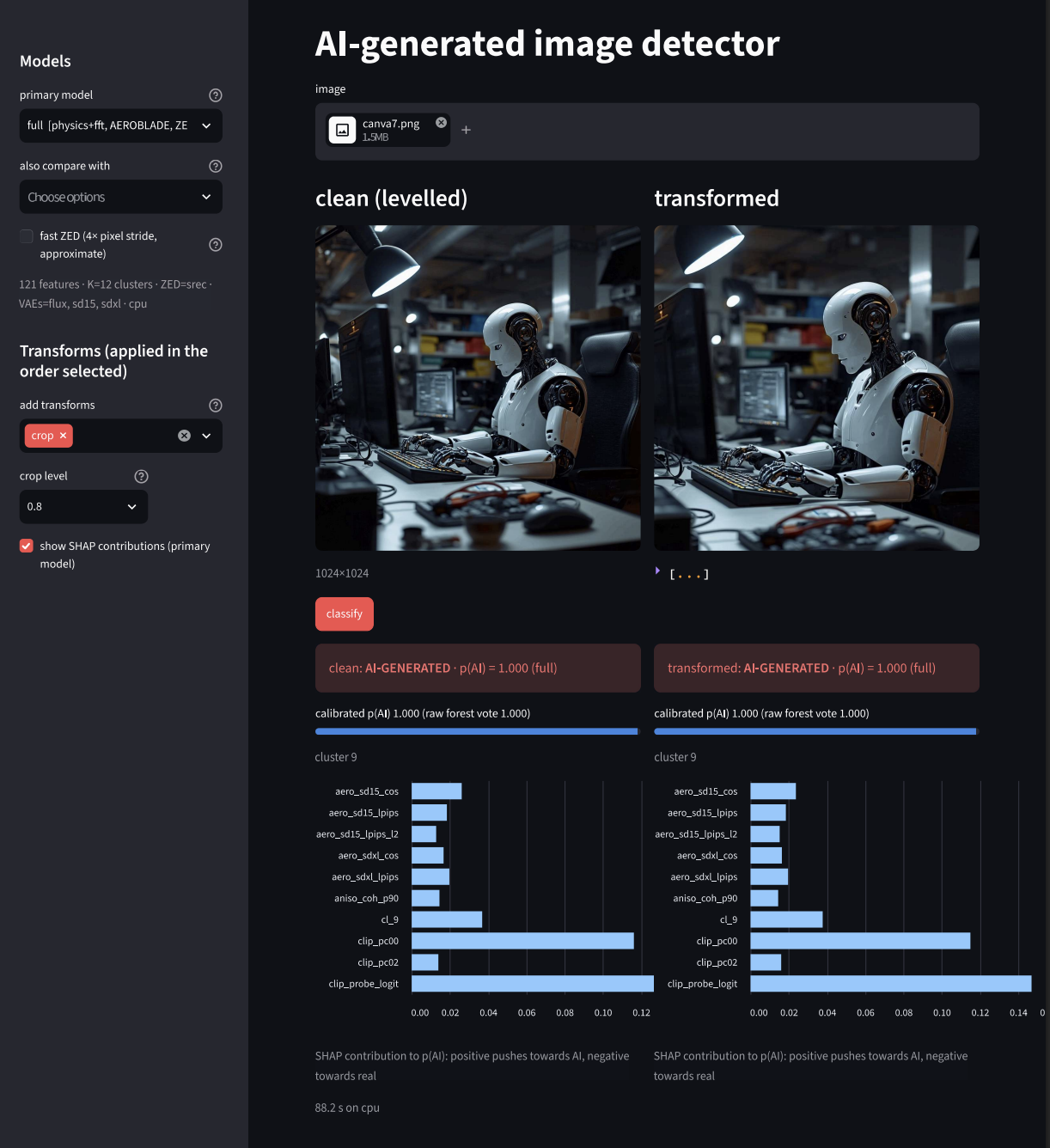
A class-balanced random forest combines them — deliberately not another neural network, so we can ask it which features matter, overall and per kind of image — and Platt scaling turns its votes into probabilities. The output includes the image's cluster and a SHAP breakdown of each feature's push toward "AI" or "real".

It ships as a command-line classifier (folder → JSON), an evaluation tool (folder + labels → every metric and calibration diagram) and a Streamlit dashboard where you upload an image, apply any of the organisers' transforms (JPEG, blur, resize, noise, colour jitter, crop), compare several model variants side by side, and see the explanation.

How we built it

Data. SID_Set (OpenImages vs FLUX), WildFake (seven real sources; GAN, diffusion and other generator families) and CIFAKE as a separate 32×32 tier. The organisers' demo subset (COCO val2017 + DALL·E 3) was held out of every fitted component and asserted disjoint.
Shortcut defences. Every image is re-encoded once as JPEG q95 at ingestion so real photos and generator PNGs share a compression history; preprocessing only ever crops at native resolution, never squash-resizes; width, height, format and source are kept as metadata but never fed to the model; the CLIP probe is cross-fitted so no training row carries a leaked score.
Robustness training. Each training image contributes a clean copy and one copy with a random transform from the organisers' table, with the transform and level recorded per row (never as an input) so accuracy can later be broken down by transform and severity.
Batched ingestion. The datasets are hundreds of GB of zips — far beyond Colab. The notebook fetches, featurises and deletes images 400 at a time, reads WildFake members straight out of 25–50 GB remote archives with HTTP Range requests, and checkpoints every batch's features to Drive so a runtime reset just resumes. The forest only ever sees the feature table, which fits in memory.
Model. Group-aware grid search (a clean/augmented pair never straddles a fold), out-of-bag scoring, Platt and isotonic calibration on a held-out split, permutation importance (overall, per correlated feature group, per cluster), feature-drift tables from the clean/augmented pairs, SHAP.
Tooling. Colab (T4) for training; VS Code, Jupyter, PyTorch, Hugging Face Transformers/Diffusers, scikit-learn, LightGBM (reference only), SHAP, OpenCV, Streamlit; Hugging Face Hub, ModelScope and Kaggle for data.

Challenges we ran into

Storage. Downloading the datasets exceeded Colab's disk before a single feature was computed. We rewrote ingestion to be batch-by-batch and, for WildFake, to read members out of the remote zips without ever downloading an archive.
GPU memory. A source-splicing step silently dropped a @torch.no_grad() decorator, so the VAEs built a full autograd graph for every crop and exhausted 15 GB on the first batch. Tracking it down took two fresh runtimes; the fix was one line plus a verification that the generated code keeps its decorators.
Library drift. Newer transformers changed what get_image_features returns; scikit-learn pickles refused to load across versions; Python 3.14 had no prebuilt wheel for the training version. Each became a pinned version, a version-proof call, or a verified re-pickling tool.
Suspiciously good numbers. An early single-source run scored AUC 1.000, and a later local evaluation got 100 % on 200 fresh images. We audited for leakage (none — verified by intersecting member paths with the training plan) and then found the real explanation: dataset shortcuts and a semantic branch that recognises "prompt-like" content.
CPU inference speed. About a minute per image on a laptop, 45 s of it in the ZED entropy computation — which led directly to the faster variants below.

Accomplishments that we're proud of

A detector whose decisions can be read: importance per feature family, per image sub-type, and per image.
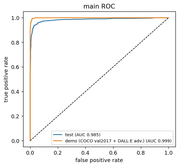
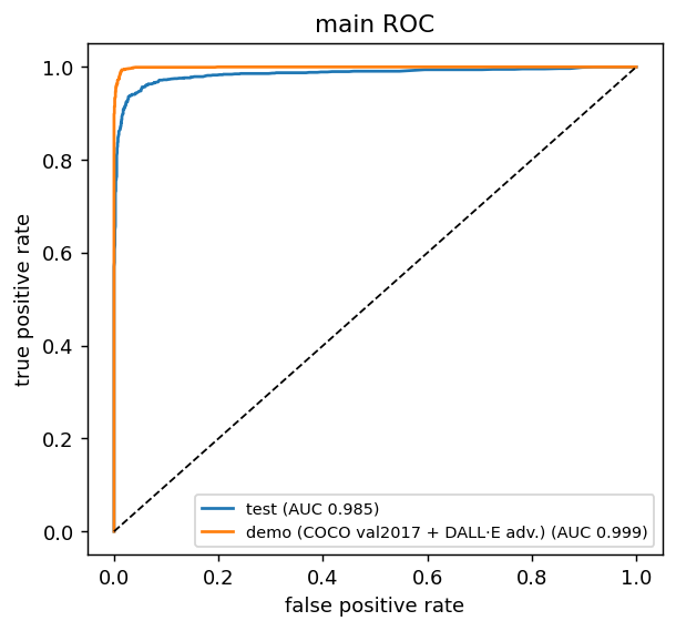
The forensic features alone are almost as good as the full model: with every CLIP-derived column removed, physics + FFT + AEROBLADE + ZED still reach AUC 0.91 on the held-out test split and 0.95 on the demo set (full model: 0.985 / 0.999). Zero or frozen parameters, each with a physical explanation.
Using that to trade accuracy for speed on purpose: dropping ZED costs < 0.001 AUC and removes most of the CPU cost; the forensics-only and no-ZED variants score several times faster with a small, known degradation. Our submission is the full model; the variants are one flag away.
Honesty tooling that we would want from any detector: a leakage test, a "hardening" script that equalises compression history and image size across classes to separate generator artefacts from dataset artefacts, and a one-command evaluation on fresh images that produces the complete metric table and calibration diagrams.
The whole training pipeline runs on a free Colab GPU, resumable, from datasets that are two orders of magnitude larger than its disk.

What we learned

Interpretability finds shortcuts. Because the forest could tell us what it used, we saw that on a single source pair CLIP alone separated the classes perfectly and kept doing so under blur that destroys every forensic cue — content, not synthesis. Multi-source training shrank that effect; the ablations quantify what remains.
"Less information" is not "less separable". Accuracy sometimes rose with transform severity, which looked impossible until we realised transforms act asymmetrically on the classes (blur removes sensor noise from photos, not from renders) and that the forest was trained on augmented rows.
Calibration and ranking are different things. Raw, Platt and isotonic probabilities share the same AUC; only the trust you can put in "0.8" changes.
The infrastructure is half the project. Range-reading zips, resumable batches, feature caches that make re-evaluating a new model variant instant — these decided what experiments we could afford to run.

What's next

Content-matched training pairs (real photos and generations from the same captions) to close the semantic shortcut for good, and the forensics-only model as the primary detector.
Evaluation on 2025–26 generators (GPT-Image, Nano Banana, Seedream, FLUX.2) via Community Forensics and Synthbuster; the tooling to build such a set is already in the kit.
Per-cluster forests so the image sub-type switches feature weights without acting as a prior; multi-crop features for large images; re-fitting calibration on a small sample from each new deployment domain.