AAMS-X: AI-Powered RF Spectrum Scan Scheduler
Adaptive Autonomous Mission Spectrum eXplorer
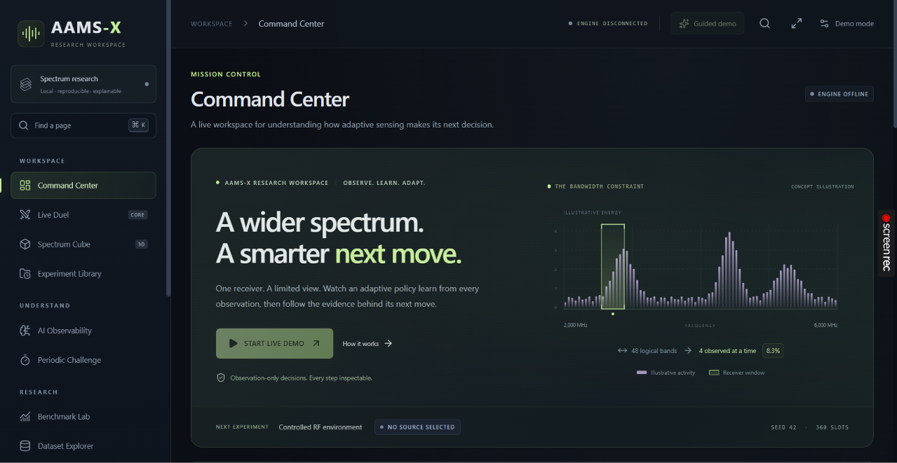
An explainable AI-powered research platform that intelligently determines where a bandwidth-limited RF receiver should scan next.
AAMS-X combines adaptive scheduling, Thompson Sampling, associative memory, information gain, periodicity estimation, and change detection to optimize RF spectrum monitoring under limited receiver bandwidth.
Inspiration
Radio-frequency (RF) spectrum monitoring is essential in electronic warfare research, wireless communication, spectrum management, and signal intelligence.
However, a fundamental challenge exists: a receiver cannot monitor the entire RF spectrum simultaneously when its instantaneous bandwidth is limited.
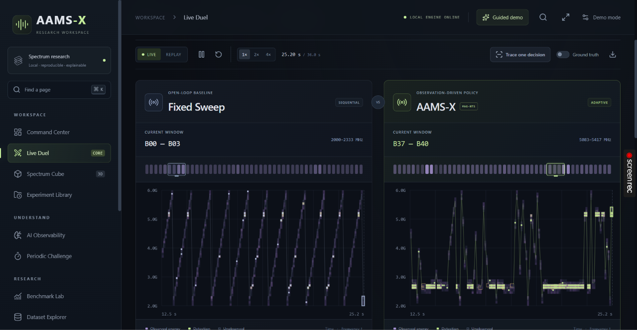
Signals can appear, disappear, and change across different frequency regions. Traditional scanning methods follow predetermined sequences, often spending valuable observation time on inactive regions while missing short-lived activity elsewhere.
This inspired us to ask:
What if an RF receiver could learn from previous observations, predict promising frequency regions, adapt to changing activity, and explain why it selected a particular frequency window?
We developed AAMS-X (Adaptive Autonomous Mission Spectrum eXplorer) to investigate this challenge.
Our objective was to build an intelligent spectrum-scanning research platform capable of:
- Identifying frequency regions with promising activity.
- Balancing exploration and exploitation.
- Learning from historical observations.
- Recognizing recurring activity patterns.
- Detecting changes in spectrum behavior.
- Minimizing unnecessary receiver retuning.
- Explaining every scheduling decision.
Rather than simply automating frequency scanning, we wanted to explore how intelligent algorithms could make spectrum monitoring more adaptive, efficient, and transparent.
What It Does
AAMS-X is an AI-powered RF spectrum scan scheduler that determines which frequency window a bandwidth-limited receiver should observe next.
The platform divides the monitored spectrum into frequency bands and selects a contiguous group of bands during each observation interval.
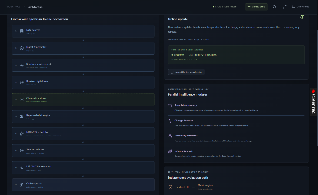
After receiving observations, the system updates its internal models and uses the accumulated evidence to determine its next scanning decision.
At its core, AAMS-X implements:
MAG-NTS: Memory-Augmented, Information-Guided Non-Stationary Thompson Sampling
MAG-NTS combines multiple techniques to support adaptive decision-making.
| Component | Purpose |
|---|---|
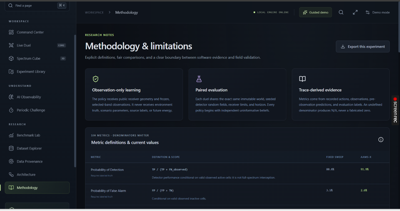
| Thompson Sampling | Balances exploration of uncertain bands with exploitation of promising bands. |
| Bayesian Activity Estimation | Maintains learned estimates of activity for individual frequency bands. |
| Information Gain | Prioritizes observations that could reduce uncertainty. |
| Associative Memory | Recognizes previously observed activity patterns. |
| Periodicity Estimation | Identifies recurring spectrum activity opportunities. |
| CUSUM Change Detection | Detects significant changes in observed behavior. |
| Revisit-Age Tracking | Encourages revisiting frequency regions that have not been observed recently. |
| Retuning-Cost Modeling | Accounts for the sensing time and movement costs associated with changing frequency windows. |
Key Features
1. Intelligent RF Spectrum Scheduling
AAMS-X continuously evaluates available frequency windows and selects the next observation region using its adaptive scheduling algorithm.
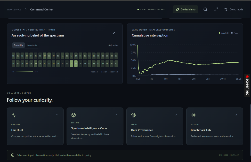
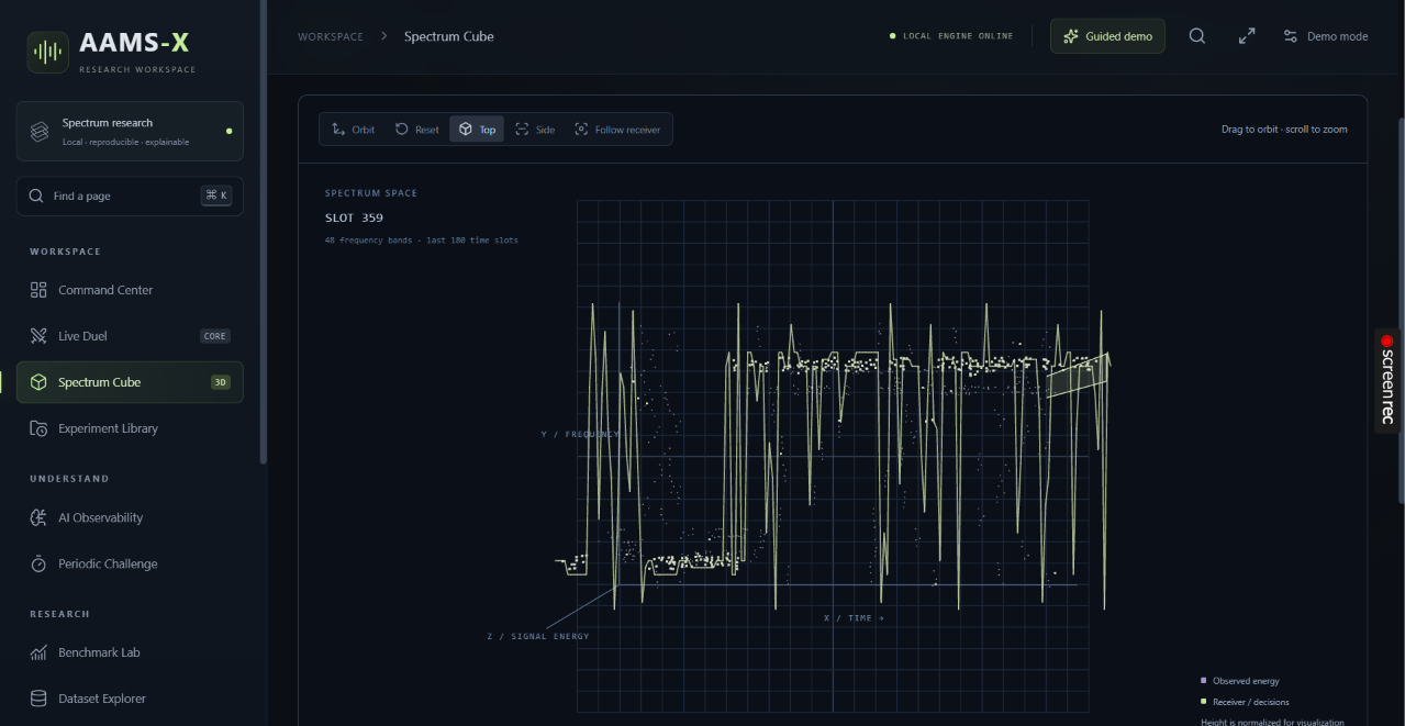
2. Interactive Spectrum Visualization
The platform provides:
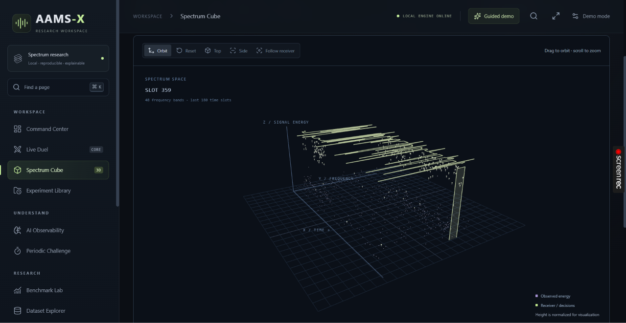
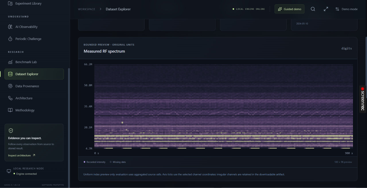
- Live spectrum waterfalls.
- Interactive 3D spectrum cubes.
- Frequency-band activity visualization.
- Scheduling timelines.
- Algorithm performance charts.
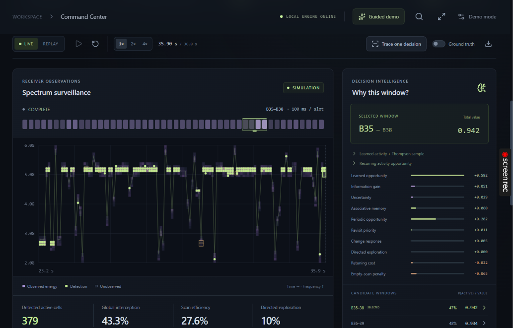
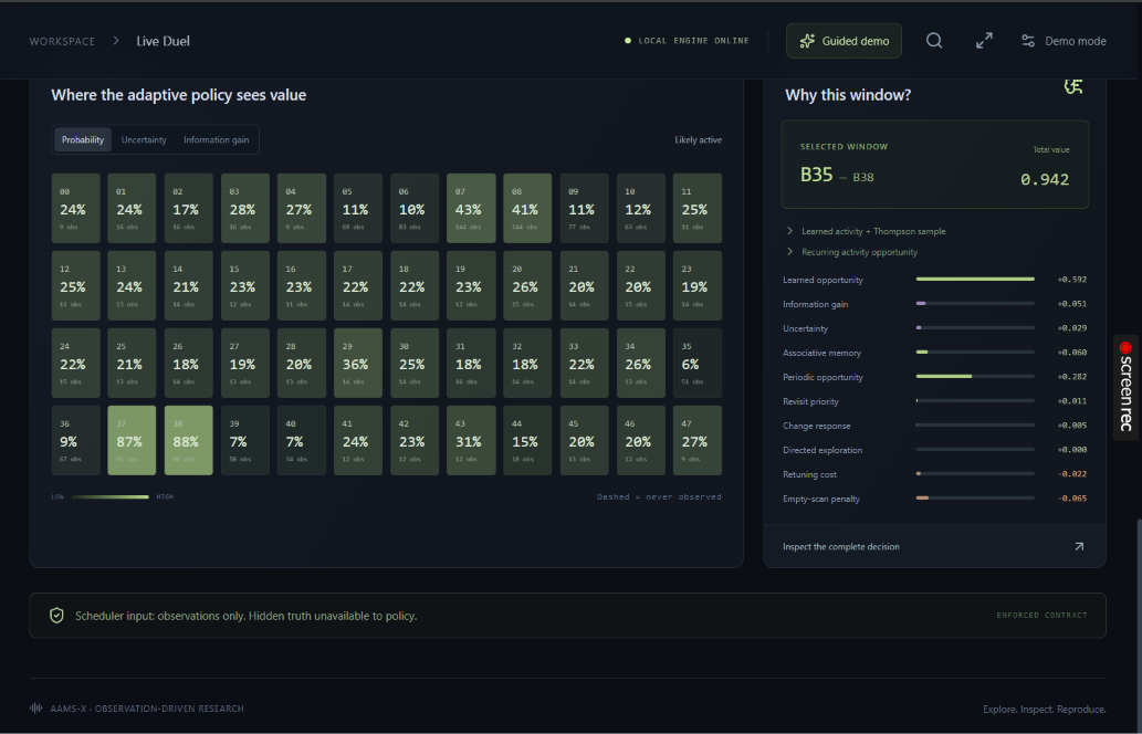
3. Explainable AI Decisions
Every scheduling decision can be inspected through:
- Estimated activity probabilities.
- Uncertainty measurements.
- Thompson Sampling contributions.
- Information-gain estimates.
- Memory-based evidence.
- Periodicity estimates.
- Retuning costs.
This enables users to understand why the scheduler selected a particular frequency window.
4. Algorithm Benchmarking
AAMS-X compares MAG-NTS against alternative scheduling approaches, including:
- Fixed-frequency sweeping.
- Vanilla Thompson Sampling.
- Algorithm ablations.
These comparisons help identify which techniques contribute to performance under different experimental conditions.
5. Dataset-Based Evaluation
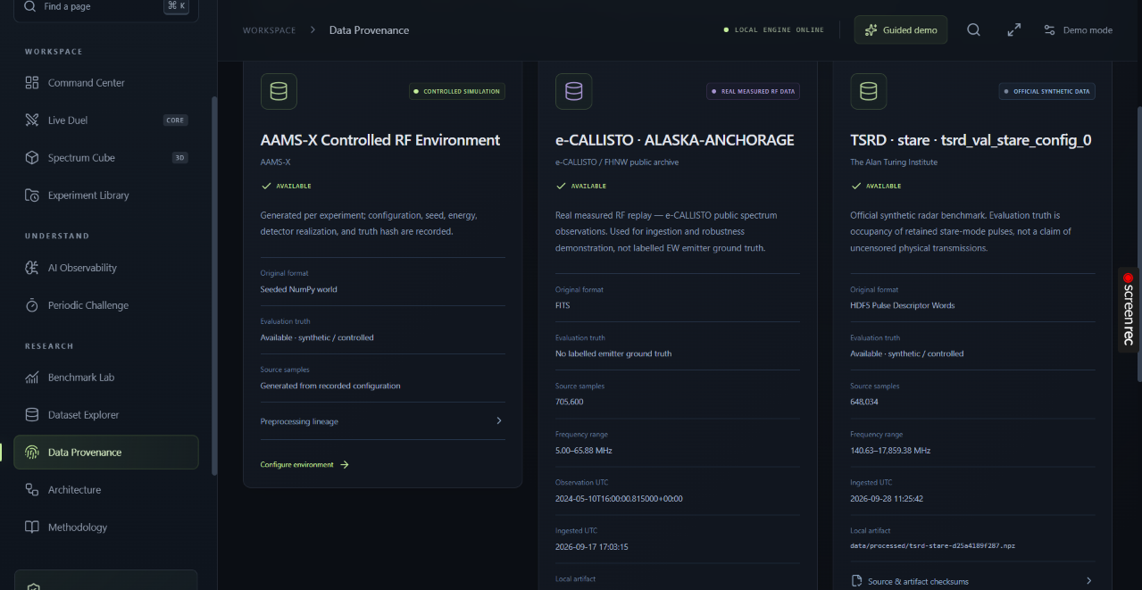
The platform supports three evaluation environments:
| Dataset/Environment | Purpose |
|---|---|
| Controlled Simulation | Evaluate scheduling behavior under configurable synthetic activity conditions. |
| Official Synthetic TSRD | Test algorithms using source-derived RF pulse occupancy. |
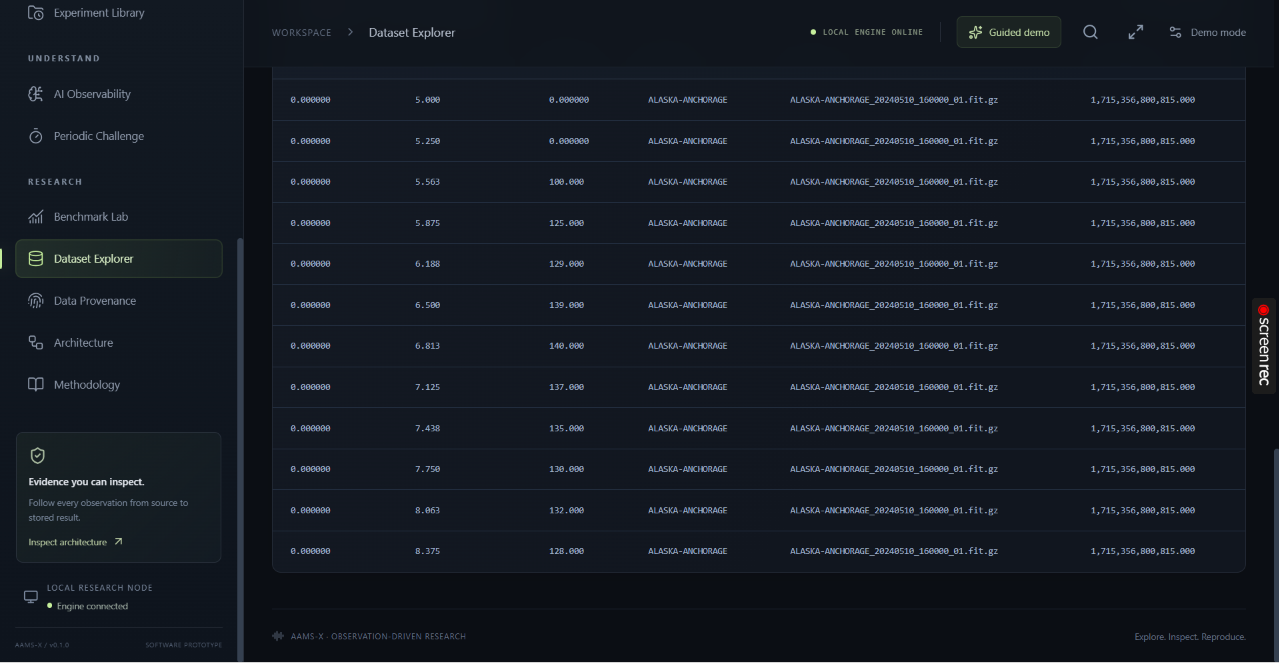
| e-CALLISTO | Explore scheduling over measured solar-radio observations. |
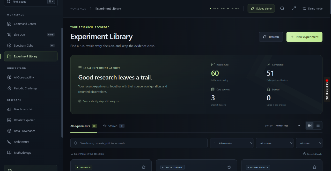
6. Experiment Replay and Reproducibility
AAMS-X allows researchers to save, export, replay, and verify experiments.
Recorded experiments include configurations, observations, scheduling decisions, and performance metrics.
How We Built It
We developed AAMS-X as a full-stack research platform integrating probabilistic learning, adaptive decision-making, receiver simulation, data processing, and interactive visualization.
1. RF Spectrum and Receiver Modeling
We first modeled the RF spectrum as a collection of discrete frequency bands.
Let:
- R: Total number of frequency bands.
- W: Number of contiguous bands observable simultaneously.
- t: Current observation time slot.
- a_t: Starting band selected by the scheduler.
- T: Total experiment duration.
The selected observation window is:
$$ \mathcal{W}(a_t)={a_t,a_t+1,\ldots,a_t+W-1} $$
The legal starting positions are:
$$ a_t\in{0,1,\ldots,R-W} $$
The observable fraction of the spectrum is:
$$ \text{Coverage Fraction}=\frac{W}{R} $$
For example, if a receiver observes four out of 64 frequency bands:
$$ \frac{4}{64}\times100=6.25\% $$
Therefore, the receiver can observe only 6.25% of the spectrum at any given time.
This makes intelligent scheduling essential.
We also implemented validation to ensure every selected observation window satisfies the receiver's bandwidth and configuration constraints.
2. Bayesian Activity Estimation
To estimate activity across frequency bands, we implemented a confidence-weighted, discounted Beta-Bernoulli model.
Each frequency band maintains two parameters:
$$ \theta_i\sim\operatorname{Beta}(\alpha_i,\beta_i) $$
Initially:
$$ \alpha_i=1,\qquad\beta_i=1 $$
The estimated activity probability is:
$$ \mathbb{E}[\theta_i]=\frac{\alpha_i}{\alpha_i+\beta_i} $$
When a band is observed, its evidence is updated based on whether the detector reports a HIT or MISS.
For confidence $c_i$:
$$ \alpha_i\leftarrow\alpha_i+c_i y_i $$
$$ \beta_i\leftarrow\beta_i+c_i(1-y_i) $$
Here:
- y_i = 1: Detected HIT.
- y_i = 0: Detected MISS.
- c_i: Observation confidence.
To adapt to changing activity, previous evidence is discounted toward the initial prior:
$$ \alpha_i^-=1+(\alpha_i-1)\lambda^{\Delta t} $$
$$ \beta_i^-=1+(\beta_i-1)\lambda^{\Delta t} $$
An important design principle is that unobserved frequency bands are never treated as inactive.
The scheduler updates its beliefs only using information the receiver actually observes.
3. Thompson Sampling for Adaptive Scheduling
We implemented Thompson Sampling to balance two competing objectives:
Exploration: Investigating frequency bands with limited or uncertain observations.
Exploitation: Revisiting bands that have previously produced useful detections.
For each band, the algorithm samples:
$$ \widetilde{\theta}_i\sim\operatorname{Beta}(\alpha_i,\beta_i) $$
These samples contribute to evaluating candidate observation windows.
Unlike fixed scanning, Thompson Sampling naturally balances learned activity estimates and uncertainty.
This allows the scheduler to adapt its scanning behavior as new observations become available.
4. Information-Guided Exploration
We integrated information gain to identify observations that could improve the scheduler's knowledge.
The uncertainty of a Beta distribution is:
$$ \operatorname{Var}(\theta_i)= \frac{\alpha_i\beta_i} {(\alpha_i+\beta_i)^2(\alpha_i+\beta_i+1)} $$
The normalized uncertainty score is:
$$ u_i=\operatorname{clip}_{[0,1]} \left(\sqrt{12\operatorname{Var}(\theta_i)}\right) $$
We also calculate the expected information gain of an additional observation under the assumed Beta-Bernoulli model.
This allows AAMS-X to consider not only which bands are promising but also which observations could be informative.
5. Associative Memory
We developed an associative-memory component that stores short observation patterns and their subsequent observed outcomes.
The system compares current observation contexts with historical episodes using:
- Pattern similarity.
- Frequency-band proximity.
- Memory age.
The retrieval weight for stored episode $j$ is:
$$ \kappa_j= s_j^4 \exp\left(-\frac{|b_j-i|}{\max(1,R/3)}\right) \exp\left(-\frac{t-t_j}{240}\right) $$
Where:
- s_j: Pattern similarity.
- b_j: Historical frequency band.
- i: Current candidate band.
- t_j: Historical observation time.
The weighted historical outcome is:
$$ \widehat{y}_i= \frac{\sum_j\kappa_j y_j} {\sum_j\kappa_j} $$
This helps the scheduler reuse evidence from similar previously observed activity patterns.
6. CUSUM-Based Change Detection
RF activity can change over time, making previously learned estimates less reliable.
To address this, we implemented a two-sided Cumulative Sum (CUSUM) detector.
The positive accumulator is:
$$ G_k^+=\max(0,G_{k-1}^++e_k-\nu) $$
The negative accumulator is:
$$ G_k^-=\max(0,G_{k-1}^--e_k-\nu) $$
Here, $e_k$ represents the difference between the observed outcome and the expected activity estimate.
When sufficient evidence indicates a change, the scheduler can increase exploration priority and reduce reliance on outdated observations.
Change detection uses only observed evidence; it cannot immediately detect activity changes outside the receiver's selected window.
7. Periodicity Estimation
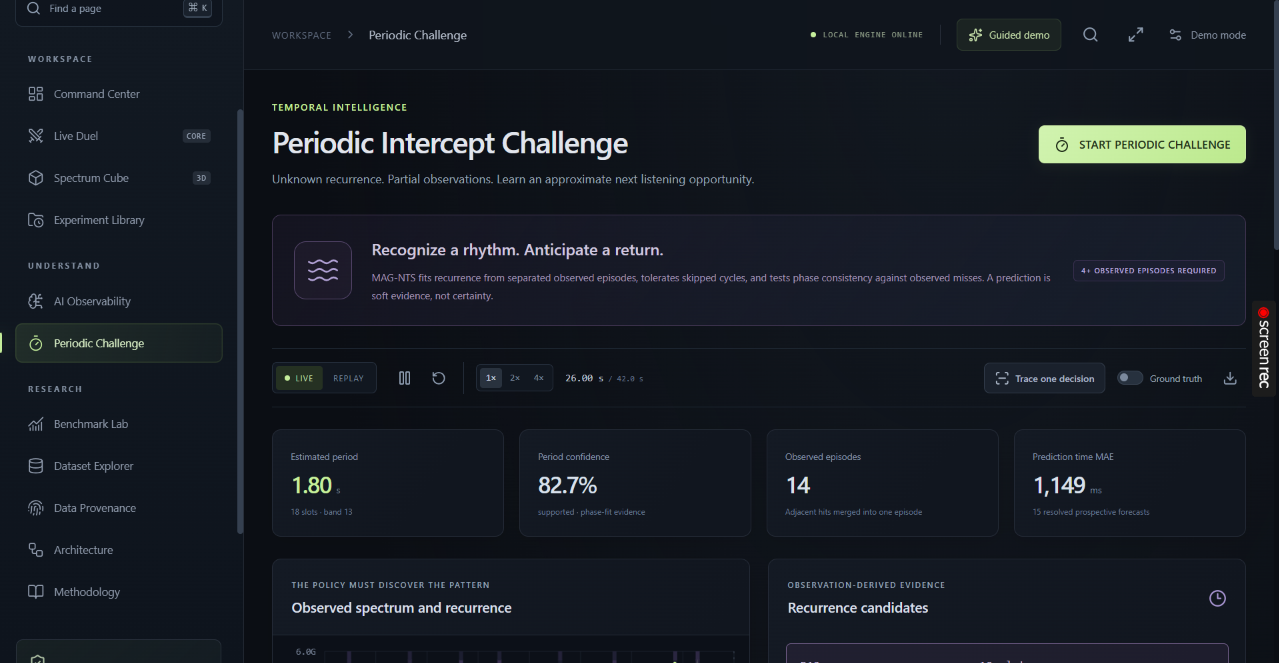
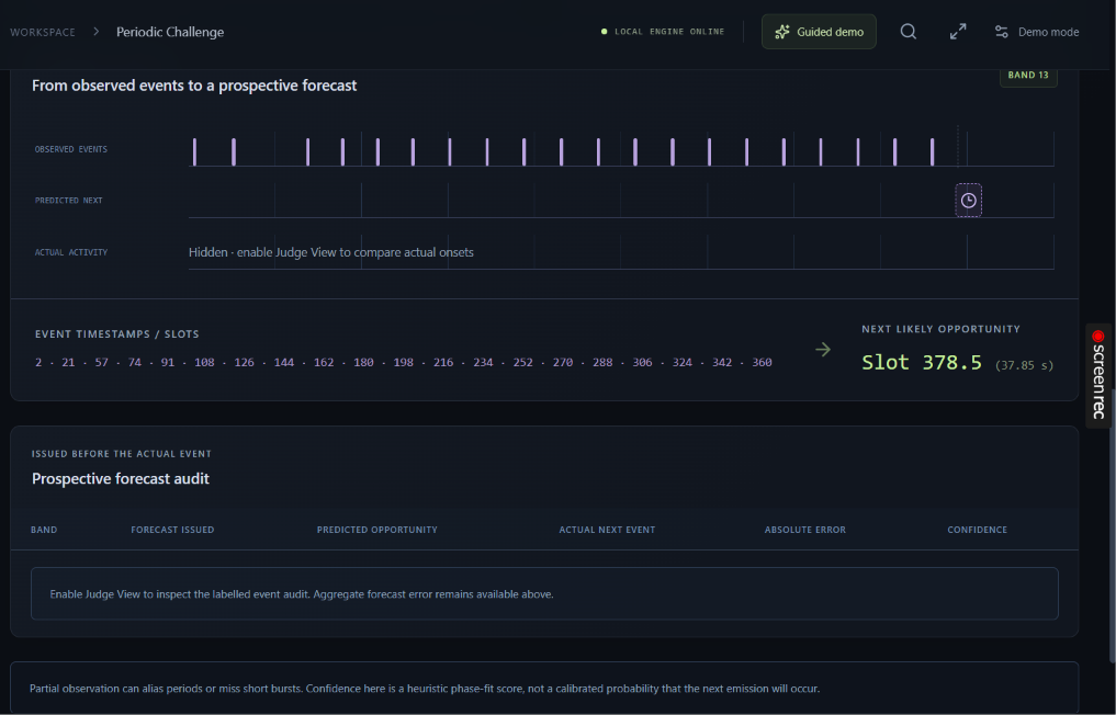
Certain frequency bands may exhibit recurring activity.
We implemented periodicity estimation to identify such patterns from separated observed activity episodes.
Given an estimated period $P$ and phase $\phi$, the next predicted opportunity is:
$$ t_{\text{next}}= \phi+ P\left\lceil\frac{t+1-\phi}{P}\right\rceil $$
This allows recurring observation opportunities to contribute to scheduling decisions.
The system also exposes tentative periodicity estimates because incomplete observations can introduce uncertainty.
8. Receiver Retuning and Timing Constraints
Changing frequency windows introduces delays that reduce available sensing time.
We modeled:
- Observation slot duration.
- Scan latency.
- Receiver retuning delay.
- Frequency movement cost.
The retuning cost is:
$$ C_t(a_t)= J_t\left[ \frac{r}{\tau} + \gamma\frac{|a_t-a_{t-1}|}{\max(1,R-W)} \right] $$
Where:
- r: Retuning delay.
- tau: Slot duration.
- gamma: Frequency movement weight.
- J_t: Indicator of whether the receiver changes windows.
This prevents the scheduler from assuming that switching frequency windows is free.
9. MAG-NTS Decision Engine
Finally, we combined the different scheduling components into a composite scoring framework.
Candidate windows are evaluated using:
- Thompson Sampling estimates.
- Information gain.
- Associative-memory evidence.
- Periodic activity opportunities.
- Revisit age.
- Change-detection priority.
- Repeated-empty-observation penalties.
- Receiver retuning costs.
The selected action is:
$$ a_t= \underset{a\in{0,\ldots,R-W}}{\operatorname{argmax}} S_t(a) $$
Where $S_t(a)$ represents the composite scheduling score for candidate window $a$.
The system records the decision components so users can inspect how the scheduler reached its selection.
10. Full-Stack Platform Development
We integrated the scheduling engine into a modern web application.
| Technology | Purpose |
|---|---|
| Python | Core scheduling algorithms and experiment logic |
| NumPy | Numerical computation |
| SciPy | Statistical calculations |
| FastAPI | Backend API |
| WebSockets | Real-time experiment updates |
| React | Interactive frontend |
| TypeScript | Type-safe frontend development |
| Three.js | 3D spectrum visualization |
| React Three Fiber | React-based 3D rendering |
| Recharts | Performance charts and analytics |
| Tailwind CSS | Responsive interface styling |
| Zustand | Frontend state management |
| SQLite | Experiment registry |
| Parquet and NPZ | Dataset storage and processing |
| Pytest | Automated backend testing |
The application connects algorithm execution, live visualization, experiment management, benchmarking, and replay into a unified research environment.
Challenges We Ran Into
1. Learning From Incomplete Observations
The biggest challenge was designing a scheduler that could make intelligent decisions without observing the entire spectrum.
Since the receiver monitors only a small frequency window at a time, activity outside that window remains unknown.
We addressed this by maintaining independent activity beliefs and ensuring that unobserved bands were never incorrectly classified as inactive.
2. Balancing Exploration and Exploitation
Repeatedly scanning promising bands can improve immediate detections but may cause the receiver to miss activity elsewhere.
Exploring unfamiliar bands improves coverage but can sacrifice opportunities in previously active regions.
We investigated this tradeoff using Thompson Sampling, information gain, revisit age, and adaptive scheduling.
3. Handling Non-Stationary RF Activity
Frequency-band activity can change over time.
A band that was previously active may become inactive, while another band may become promising.
We integrated discounted Bayesian evidence and CUSUM change detection to help the scheduler respond to changing observations.
4. Distinguishing Detection Performance From Scheduling Performance
One important challenge was defining appropriate evaluation metrics.
A receiver may achieve high detection performance within the frequency window it observes while missing substantial activity elsewhere.
We therefore distinguished conditional detection probability from global spectrum recall.
Conditional detection probability:
$$ P_D=\frac{TP}{TP+FN_{\text{observed}}} $$
Global recall:
$$ \operatorname{Recall}= \frac{\sum_t TP_t}{\sum_t N_{\text{active},t}} $$
This distinction helped us evaluate whether an algorithm actually improved spectrum coverage.
5. Ensuring Fair Algorithm Comparisons
Different scheduling algorithms must operate under comparable experimental conditions.
We implemented paired evaluations using shared underlying activity, receiver constraints, timing configurations, and detector realizations.
Each algorithm maintains its own learning state while operating in the same experimental world.
This makes comparisons more meaningful.
6. Working With Different Dataset Types
Synthetic and measured RF datasets provide different forms of evidence.
We worked with controlled simulation, official synthetic TSRD data, and measured e-CALLISTO observations.
A key challenge was ensuring that evaluation claims remained consistent with the available ground truth.
For example, the included e-CALLISTO recording does not provide labeled emitter truth, so truth-dependent detection metrics are unavailable for that source.
7. Building an Explainable Real-Time Interface
Integrating adaptive scheduling algorithms with interactive 3D visualization, live updates, and experiment replay required coordination between the backend and frontend.
We addressed this through FastAPI, WebSockets, React, Three.js, and structured experiment traces.
Accomplishments That We're Proud Of
1. Developed a Complete Adaptive RF Spectrum Research Platform
We successfully integrated:
- Adaptive RF spectrum scheduling.
- Probabilistic activity estimation.
- Thompson Sampling.
- Information-guided exploration.
- Associative memory.
- Periodicity estimation.
- Change detection.
- Receiver timing constraints.
- Explainable scheduling decisions.
- Interactive 3D visualization.
- Reproducible algorithm benchmarking.
The result is a research platform that makes scheduling decisions both observable and explainable.
2. Evaluated MAG-NTS Using Official Synthetic TSRD Data
Our documented evaluation included:
| Evaluation Parameter | Value |
|---|---|
| Retained RF pulses | 648,034 |
| Paired experimental worlds | 24 |
| Policy evaluations | 192 |
| Algorithms and ablations | 8 |
| Random seeds | 42-47 |
| Receiver bandwidth configurations | 4 |
| Time slots per world | 240 |
Global Recall Comparison
| Observable Bandwidth | Fixed Sweep | MAG-NTS | Vanilla Thompson Sampling |
|---|---|---|---|
| 2 / 64 bands | 2.71% | 13.27% | 15.83% |
| 4 / 64 bands | 5.47% | 31.48% | 36.75% |
| 8 / 64 bands | 11.07% | 37.38% | 39.55% |
| 16 / 64 bands | 21.96% | 52.34% | 55.30% |
At a receiver bandwidth of four out of 64 bands:
Fixed Sweep Recall: 5.47%
MAG-NTS Recall: 31.48%
The absolute improvement is:
$$ 31.48\%-5.47\%=\boxed{26.01\text{ percentage points}} $$
This corresponds to approximately:
$$ \frac{31.48}{5.47}\approx\boxed{5.75\times} $$
MAG-NTS achieved approximately 5.75 times the global recall of fixed sweeping under this evaluated configuration.
Importantly, Vanilla Thompson Sampling achieved higher recall than MAG-NTS in these experiments.
This reinforced the importance of transparent benchmarking rather than assuming that more complex algorithms always perform better.
These results come from one synthetic validation recording with modeled receiver noise and do not establish real-world hardware performance.
3. Built Explainable Scheduling Decisions
Instead of presenting only the selected frequency window, AAMS-X exposes the evidence contributing to each decision.
Users can inspect activity estimates, uncertainty, information gain, memory contributions, periodicity, and retuning costs.
This makes the platform useful for understanding and evaluating adaptive scheduling behavior.
4. Implemented Reproducible Experiments
We developed an experiment registry that records:
- Experiment configurations.
- Receiver observations.
- Algorithm decisions.
- Performance metrics.
- Replay traces.
Trace integrity is verified using SHA-256 checksums.
This supports reproducibility and helps identify accidental data corruption.
5. Validated the Application
The repository documents:
- 36 passing backend tests.
- Successful TypeScript checks.
- Successful production frontend builds.
- Receiver-constraint validation.
- Deterministic experiment reruns.
- API and WebSocket testing.
- Replay-integrity verification.
- Documented browser workflow testing.
What We Learned
1. Simpler Algorithms Can Outperform More Complex Ones
One of our most important findings was that adding more components does not automatically improve performance.
Although MAG-NTS combines memory, periodicity, information gain, and change detection, Vanilla Thompson Sampling achieved higher global recall in the documented TSRD evaluation.
This taught us the importance of strong baselines, ablation studies, and evidence-based algorithm development.
2. Unobserved Does Not Mean Inactive
A receiver cannot infer that a frequency band is inactive simply because it was not observed.
Maintaining this distinction is essential for accurate belief updates, change detection, and evaluation.
3. Exploration Is Essential Under Limited Bandwidth
When only a small fraction of the spectrum can be monitored, repeatedly observing the same regions can result in missed opportunities elsewhere.
Adaptive exploration helps distribute observations more intelligently.
4. Realistic Receiver Constraints Matter
Retuning and scan latency reduce usable sensing time.
Ignoring these costs can make frequently switching algorithms appear more effective than they would be under realistic timing constraints.
We learned to incorporate these limitations directly into the experimental model.
5. Explainability Improves Algorithm Development
Understanding why a scheduler selects a particular frequency window is valuable for debugging and research.
By exposing component-level scores, we can investigate whether decisions are driven by reliable evidence, uncertainty, historical patterns, or potentially misleading estimates.
6. Evaluation Metrics Must Be Interpreted Carefully
High detection probability within observed windows does not necessarily imply high global spectrum recall.
Similarly, results from synthetic datasets cannot automatically be generalized to measured RF environments.
This project strengthened our understanding of experimental methodology, reproducibility, and responsible interpretation of results.
What's Next for AAMS-X: AI-Powered RF Spectrum Scan Scheduler
We envision AAMS-X evolving from a software research prototype into a broader experimental platform for adaptive spectrum sensing.
1. Software-Defined Radio Integration
Integrate AAMS-X with calibrated Software-Defined Radio (SDR) hardware to study scheduling under actual receiver acquisition and tuning constraints.
2. Hardware-in-the-Loop Testing
Evaluate the scheduler using real receiver timing, acquisition behavior, and bandwidth limitations.
3. Expanded Dataset Evaluation
Test additional synthetic and measured RF recordings to understand how well the scheduling approaches generalize across different activity patterns.
4. Multi-Receiver Coordination
Explore cooperative scheduling in which multiple receivers share selected information and coordinate their spectrum coverage.
5. Advanced Learning Algorithms
Investigate additional approaches for partially observable and non-stationary environments, including policies that use longer observation histories.
6. Edge AI Deployment
Study the feasibility of running adaptive scheduling algorithms on resource-constrained edge devices.
7. Longer-Duration Experimental Evaluation
Evaluate scheduling stability, computational overhead, memory consumption, and adaptation over extended experimental runs.
Our long-term goal is to make AAMS-X a transparent, reproducible platform for researching intelligent RF spectrum sensing and adaptive receiver scheduling.
Built With
Python FastAPI NumPy SciPy React TypeScript Three.js React Three Fiber Recharts Tailwind CSS Zustand SQLite WebSockets Apache Parquet Vite Pytest
Try It Out
Live Application:
https://13-203-47-246.sslip.io
GitHub Repository:
https://github.com/Siddhanthkjain2005/AAMS-X
Project Summary
AAMS-X transforms RF spectrum scanning from a predetermined sequence into an adaptive, evidence-driven decision process.
By combining probabilistic learning, Thompson Sampling, associative memory, information gain, periodicity estimation, and change detection, the platform investigates how bandwidth-limited receivers can allocate their observation time more effectively.
With explainable decisions, interactive 3D visualization, reproducible benchmarking, and dataset-based evaluation, AAMS-X provides a foundation for further research into intelligent spectrum monitoring.
AAMS-X — Observe intelligently. Learn continuously. Explore adaptively.
Built With
- apache-parquet
- fastapi
- numpy
- pytest
- python
- react
- react-three-fiber
- recharts
- scipy
- sqlite
- tailwind-css
- three.js
- typescript
- vite
- websockets
- zustand

Log in or sign up for Devpost to join the conversation.