Robust AIGC Detection

New Experimented Pipeline (Generalisation)

Inspiration

As generative AI models become increasingly capable of producing photorealistic images, distinguishing between real and AI-generated content is becoming more difficult. This creates challenges for misinformation, content authenticity, and trust in digital media.

Our project, Robust AIGC Detection, explores how machine learning can be used not only to detect AI-generated images, but also to remain reliable when encountering images from generators and conditions that were not seen during training.

What it does

Robust AIGC Detection is a machine learning system that classifies an image as either real or AI-generated.

Rather than focusing only on performance on a single dataset, we investigate three important aspects of AI-generated image detection:

Generalisation — detecting images produced by generators that were not seen during training.
Robustness — maintaining detection performance after common image transformations and distortions.
Hybrid detection — investigating whether complementary detection signals can improve overall detection reliability.

Each approach is evaluated against a common baseline so that we can determine whether the additional techniques provide meaningful improvements.

How we built it

Baseline

We first developed a common baseline that could be used as a consistent reference point for the team's subsequent experiments.

Our baseline detector was built using PyTorch and Hugging Face Transformers, with the pretrained SigLIP2 Base (ViT-B/16 @256) model as a frozen image encoder.

The baseline architecture is:

Input Image → SigLIP2 Image Encoder → 768-dimensional Image Representation → Binary Linear Classifier → P(AI)

The SigLIP2 backbone was kept frozen during training, while a binary linear classification head was trained to distinguish between real and fully AI-generated images.

For training, we used SID_Set with the following labels:

0 — Real image
1 — Fully AI-generated image
2 — Tampered/AI-edited image (excluded)

We constructed a balanced subset of real and fully AI-generated images and used a fixed random seed with a consistent train/validation split to make the experiments reproducible.

Our baseline training pipeline includes:

Balanced sampling of real and AI-generated images
Reproducible train/validation splitting
Image preprocessing using the SigLIP2 processor
Binary classification using BCEWithLogitsLoss
Optimisation using AdamW
Evaluation using ROC-AUC
Model checkpointing based on validation performance

The trained baseline outputs a continuous P(AI) score between 0 and 1, where a higher value indicates that an image is more likely to be AI-generated.

The baseline model, training pipeline, and checkpoint format then served as the common foundation for the team's subsequent experiments.

Generalisation

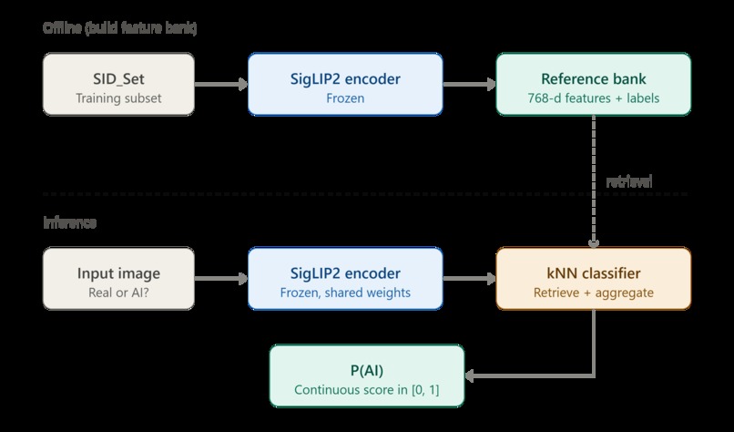
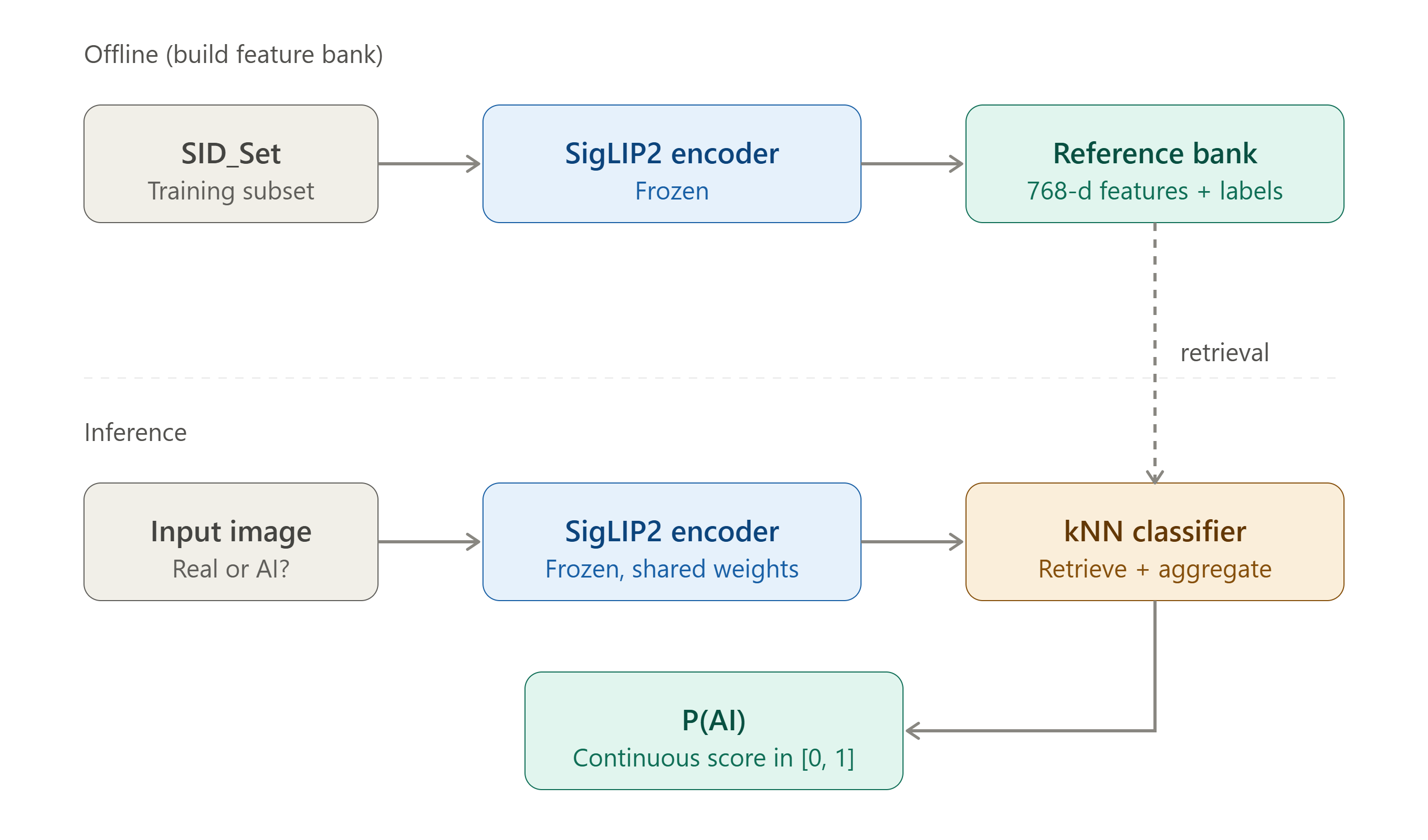
For our generalisation experiment, we investigated whether a non-parametric nearest neighbour classifier on frozen SigLIP2 features could match or exceed the linear probe baseline when tested on unseen generators.

We kept the SigLIP2 backbone, preprocessing, and training data identical to the baseline, but replaced the trained linear classification head with a k-Nearest Neighbours (kNN) classifier operating directly on the 768-dimensional frozen features.

Instead of being used to fit a classifier, the balanced SID_Set training subset was encoded once with the frozen SigLIP2 encoder and stored as a reference feature bank. At inference time, an input image was encoded, its nearest neighbours in the bank were retrieved, and their labels were aggregated into a continuous P(AI) score.

Why the approach was tested

We took inspiration from UnivFD (Ojha et al., 2023), which showed that a nearest neighbour rule on frozen CLIP features could serve as a competitive AI-image detector without training any parametric head. Our hypothesis was that kNN might actually be a better fit for SigLIP2 than for the CLIP encoder UnivFD originally used, for two reasons.

Sigmoid pairwise loss instead of softmax contrastive. CLIP's contrastive objective relies on global batch statistics, whereas SigLIP replaces this with a sigmoid loss over independent image text pairs that encourages more informative local feature geometry. Since kNN depends entirely on local neighbourhood structure, this seemed like a natural match.
Additional self-supervised objectives in SigLIP2. SigLIP2 augments the sigmoid loss with self distillation and masked prediction, producing features that are denser and more locally coherent than CLIP's contrastive-only features, giving a nearest neighbour rule more signal to work with.

If the hypothesis held, a kNN head on SigLIP2 would give us a generalisation-friendly detector without training any parameters on the detection task, a strong result for unseen generators like DALL·E Advanced in the WildFake subset.

Results

Method	External ROC-AUC (WildFake subset)
Baseline (frozen SigLIP2 + linear probe)	0.9751
Ours (frozen SigLIP2 + kNN)	0.8560

The nearest-neighbour variant underperformed the linear probe by roughly 11 AUC points on the external evaluation.

What we learned

Our hypothesis did not hold. Despite SigLIP2's arguably kNN-friendlier training regime, the linear probe still clearly outperformed nearest neighbour, mirroring an ablation reported in UnivFD itself on CLIP. The real vs AI signal in the SigLIP2 feature space appears to be captured by a globally consistent linear direction that a trained linear head can exploit but local neighbourhood similarity does not fully recover. Better local geometry from the sigmoid loss and self-supervised objectives is not enough to close that gap.

More broadly, this experiment reinforced a central takeaway of the project. For this task, backbone quality dominates over head architecture. A strong frozen backbone with a trivial linear head already provides most of the generalisation benefit, and swapping to a non-parametric head does not unlock additional generalisation, it costs performance.

We kept the linear probe as the head for our production model and treated the kNN experiment as an informative ablation. It clarifies where the detection signal lives in the SigLIP2 feature space and rules out non-parametric retrieval as a cheap route to better generalisation on unseen generators.

Robustness

To test whether training-time augmentation improves the detector's resilience to real-world image degradation without hurting clean-image accuracy, four training strategies were compared: R0 (no augmentation, clean-image baseline), R1 (one randomly chosen corruption applied per training image), R2 (a fixed composite pipeline: JPEG compression → Gaussian blur → resize round-trip, applied to every training image), and R3 (1–2 randomly chosen corruptions per training image). All four were trained under identical conditions (1000 samples/class, 1 epoch, batch size 4, seed 42) so results are directly comparable.

Each resulting checkpoint was scored on the same held-out SID_Set validation split under 14 fixed perturbation conditions spanning 7 categories — clean, JPEG (q=90/70/50/30), Gaussian blur (σ=0.5/1.0/2.0), resize round-trip (0.5x/0.25x), Gaussian noise (σ=0.02/0.05/0.10), colour jitter, and center crop (80%) and a clean-only pass on an external WildFake subset to check for generalisation

Results

Model	Clean	JPEG	Blur	Resize	Noise	Colour	Crop	Robust Mean	External
R0	0.9985	0.9967	0.9978	0.9982	0.9915	0.9987	0.9992	0.9970	0.9751
R1	0.9987	0.9971	0.9981	0.9985	0.9940	0.9986	0.9991	0.9976	0.9814
R2	0.9985	0.9971	0.9981	0.9986	0.9938	0.9986	0.9989	0.9975	0.9871
R3	0.9984	0.9970	0.9980	0.9983	0.9939	0.9981	0.9990	0.9974	0.9827

Compared with the baseline (R0)

Every augmented strategy improves on R0's robust mean and there is a larger improvement on external generalisation in which R2 external AUC is 0.9871, an increase of 0.012 from R0's 0.9751. Gaussian noise is the hardest internal condition for all four strategies (the lowest column across the board), but augmentation training closes most of that gap: R0 sits at 0.9915 vs. ≥0.9938 for R1/R2/R3.

Clean vs. robustness trade-off

Clean-image accuracy barely changes across strategies (0.9984–0.9987, a 0.0003 spread) showing that the augmentation does not have a drastic effect on clean images. Internally, the four strategies are also very close on robust mean (≤0.0006 apart). External generalisation is where the strategies have a more evident separation (a 0.012 spread), making it the more decision-relevant signal.

Best-performing strategy

R1 has the best clean AUC (0.9987) and best internal robust mean (0.9976), making it the strongest choice if the deployment distribution closely resembles SID_Set. R2 has the best external AUC (0.9871) by a clear margin, at negligible cost to clean/internal-robust performance.

Why R2 was selected as the final strategy

Internal metrics are close to indistinguishable across R1/R2/R3, making them a slightly weaker metrics for selection. External generalisation is the metric that differentiates the strategies more evidently and provide a clearer idea on how the model will perform on images that it was not been trained, which is the scenario robustness testing is meant to guard against in the first place. R2's fixed JPEG→blur→resize composite mirrors the kind of degradation real-world images typically undergo (re-compression, resizing, mild blur from re-encoding), which likely explains why it generalises best despite being the least "randomised" of the three augmented strategies. R0 was ruled out as it is dominated by every augmented strategy on both robust mean and external AUC, with no offsetting clean-AUC advantage.

Hybrid Detection

To improve the model's ability to learn features resulting from AI generation instead of relying on semantic cues, we experimented with incorporating patch shuffling, during which the input image is split into patches which are then shuffled, into the pipeline. Specifically, we experimented with two approaches: 1) a dual branch architecture where the input image is passed into one branch while a patch-shuffled version of the same image is passed into the other branch, and 2) our baseline model with patch shuffling as data augmentation.

For the first approach, the same pre-trained SigLIP2 backbone that was used in our baseline model was used as the backbone for both branches. After both the original input image and its patch-shuffled counterpart go through the backbone, their embeddings are concatenated and passed as input to the classifier head.

For the second approach, our baseline model was used with the addition of patch shuffling as a data augmentation strategy. Patch shuffling was only applied to images in the training set with a probability of 0.5. The rest of the pipeline follows that of the baseline model.

Results

The first approach achieved similar results to the baseline model but with twice the inference time. Hence, we did not incorporate the dual branch architecture into our final model.

The second approach achieved a slightly lower AUC than the baseline model on our internal test set:

Method	Internal AUC
Baseline	0.9985
Patch-shuffle	0.9928

Hence, we did not incorporate patch shuffling as data augmentation in our final model.

What we learned

Though our experiments showed that patch augmentation did not improve our model, this is likely due to flaws in our implementation. Approaches to AI-generated image detection involving patch shuffling have been shown to have good results; for example, Zheng et al. (2024) and Yang et al. (2025). These approaches used more complicated architectures than ours, such as utilising a self-attention layer in the case of Yang et al. (2025). It is likely that our relatively simple implementations of patch shuffle integration were inadequate for taking advantage of the benefits of patch shuffling.

Evaluation and Error Analysis

Methodology

Evaluation was run through the common P5 evaluator (evaluator.py, transforms.py, run_evaluation.py), shared across baseline, P2, P3, and P4 so results are directly comparable. For a given checkpoint, run_full_combined_evaluation runs inference across all 14 transform conditions defined in TRANSFORM_CONDITIONS on the held-out SID_Set validation split, computes ROC-AUC per condition (evaluate_condition), and aggregates into the 7 result-table categories (summarize_by_group): clean, JPEG, blur, resize, noise, colour, crop. The same checkpoint is separately scored on the provided WildFake subset (COCO real vs. DALL·E Advanced), per the rule that this set must never appear in training.

The evaluator also implements the analysis functions: find_hardest_condition, compute_degradation / find_biggest_degradation, jpeg_trend, internal_external_gap, and get_false_positives_negatives (which returns sorted false-positive/false-negative lists with image path, label, and predicted score). Per-image results are saved by run_evaluation.py to a JSON file (results/{model_name}_conditions.json), with each prediction stored as an image_path / pred pair per condition.

Baseline vs. final model

Model	Clean	JPEG	Blur	Resize	Noise	Colour	Crop	Robust Mean	External
Baseline (R0)	0.9985	0.9967	0.9978	0.9982	0.9915	0.9987	0.9992	0.9970	0.9751
Final (R2)	0.9985	0.9971	0.9981	0.9986	0.9938	0.9986	0.9989	0.9975	0.9871

Clean-image AUC is unchanged between baseline and final model; the improvement is concentrated in external generalisation, which is why R2 was selected over R1/R3 despite the three augmentation strategies being close to indistinguishable internally (see Robustness section).

Hardest condition and degradation by group

Gaussian noise is the weakest internal category for all four strategies tested (R0–R3), per the Robustness section table. compute_degradation (clean AUC minus each group's AUC) confirms this for R2: noise shows the only degradation worth noting, at −0.0046 relative to clean, versus −0.0014 for JPEG and −0.0003 for blur. Resize, colour, and crop all come out negative (i.e. marginally above clean AUC: −0.0001, −0.0002, and −0.0005 respectively), which is noise rather than a real robustness gain, but underlines that noise is the only condition R2 meaningfully struggles with. find_biggest_degradation selects "noise" accordingly.

Within JPEG specifically, jpeg_trend shows AUC degrading smoothly as compression gets more aggressive (q90: 0.9980, q70: 0.9971, q50: 0.9967, q30: 0.9966), a 0.0014 drop from lightest to heaviest compression, much smaller than the noise degradation.

Error analysis

Errors were inspected using get_false_positives_negatives on the per-image predictions saved for each condition.

Internal (SID_Set, clean): the final model makes very few mistakes with 10 false positives (real images flagged as AI, most confidently at 0.76 and 0.70) and only 2 false negatives. Errors skew toward over-flagging real images rather than missing generated ones.

Internal (hardest condition): the error pattern flips. There are 0 false positives but 39 false negatives, shwoing that under heavy noise the model doesn't get fooled into calling real images "AI," it instead becomes under-confident on genuinely AI images (several dropping to a predicted P(AI) below 0.16). This suggests noise suppresses the AI-generation cues the model relies on rather than introducing spurious ones, costing recall on AI images specifically rather than raising the false-alarm rate.

External (WildFake): 72 false positives (7.2% of real COCO images misclassified, some with high confidence up to 0.88) and 48 false negatives (4.8% of AI images missed). Notably, every false negative comes from the DALL·E Advanced subset, showing that the model's confidence collapses specifically on this unseen generator (predictions as low as 0.13), while its false positives are spread across ordinary real photos. This is consistent with the ~0.0113 internal-to-external AUC gap reported above: the residual generalisation gap is concentrated in missed detections on the generator that wasn't seen during training, rather than in a general rise in false alarms.

Challenges we ran into

One challenge was the computational requirement of training and evaluating large vision models on consumer hardware. Memory limitations meant that we had to carefully design our training pipeline and share trained checkpoints across the team.

Another challenge was ensuring that improvements on one evaluation condition did not come at the expense of another. A detector may perform extremely well on images from a familiar distribution while performing worse on unseen generators or transformed images.

This meant that we could not select approaches based only on their performance on the training or validation distribution. We needed to evaluate each experiment consistently across clean, transformed, and external data.

Accomplishments that we're proud of

We developed a reproducible end-to-end detection pipeline covering dataset preparation, model training, validation, checkpointing, and external evaluation.

Our frozen SigLIP2 baseline with a simple linear classifier achieved an external ROC-AUC of 0.9751 on the WildFake subset, giving us a strong starting point for further experimentation.

We also structured the project so that generalisation, robustness, and hybrid approaches could be evaluated against the same baseline. This allowed us to determine whether additional complexity actually resulted in meaningful improvements rather than assuming that a more complex model would necessarily perform better.

What we learned

We learned that evaluating an AI-generated image detector requires looking beyond performance on familiar data. Generalisation to unseen generators and robustness to image transformations are important when considering how such a detector would perform under real-world conditions.

Our experiments also showed the importance of comparing new approaches against a strong and consistent baseline. Increasing model complexity does not necessarily lead to better performance, making controlled experiments and ablation studies important when deciding which components should be included in the final system.

We also gained practical experience working with pretrained vision models, PyTorch training pipelines, robustness evaluation, checkpoint management, and collaborative machine learning experimentation.

What's next

Given more time, we would evaluate the detector against a wider range of unseen AI image generators and real-world image transformations.

We would also investigate additional methods for improving robustness and generalisation while keeping the detector computationally efficient. This would help explore whether stronger performance can be achieved without significantly increasing training or inference costs.

Another direction would be to pair the classifier with a vision-language model to generate human-readable rationales for its predictions, improving interpretability and user trust in downstream moderation or forensic settings.