Members: Bader Alabdulrazzaq (balabdul), David Young (dyoung13), Jacob Frausto (jfraust2)

Full Final Report/Reflection

Introduction

Learning under supervision has had a profound impact in the progress of AI and machine learning over the past decades. Supervised learning, however, requires a large amount of data to achieve reasonable performance for a given task. Collecting and labelling the amount of data necessary to train supervised models is expensive and doesn’t scale well. For example, ImageNet with its 14 million images is estimated to take ~19 human years to annotate [1], keeping in mind that the dataset: has limited concepts of the world; doesn’t include any temporal concepts; and is unbalanced and not fully inclusive [2]. In many real-world scenarios, we simply don’t have access to labels for the data (e.g. machine translation for languages that aren’t as prevalent in digital form). Medical imaging is notorious for this [3] as professionals have to spend countless hours looking at images in order to manually classify and segment them.

Self-supervised learning--where a model would generate the labels needed for learning semi-automatically from the data itself-- has made tremendous progress over the past few years, with successes in NLP [4] and in video and language representation learning [5].

In this project, we’ll implement a contrastive self-supervision model to learn image representations from unlabelled data and investigate its performance for an image classification downstream task. The overall outlined learning framework is semi-supervised and trained in two stages. First we’ll implement SimCLR to extract image feature representations without using labels. Then, we’ll use a small, labeled dataset to train a classifier on top of our learned feature backbone for the classification task.

Methodology

The SimCLR model consists of a ResNet-50 feature backbone (with classification head removed) and a linear projection head g(). After training the contrastive model, we would discard the projection head and add an appropriate classification head for the downstream task. The training procedure, shown in Fig. 1, relies heavily on image augmentation to produce a pair for each sample datapoint. Those pairs, called positive samples, are the basis for the contrastive learning objective where we optimize our model to produce representations that achieve high similarity between the positive pairs and low similarity with all the other augmented data points (negatives). For the model to succeed in this objective, it would need to discover the underlying structure of the data distribution, which is what we want for our feature representation.

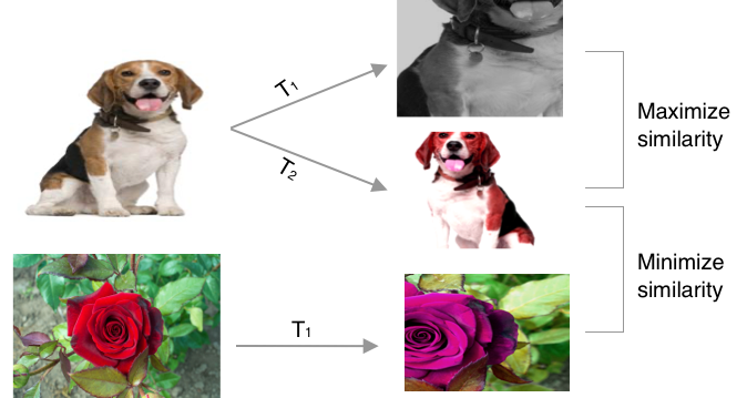
Figure 1: Diagram of the loss objective

For the augmentation process, we follow the original paper and use: random crop, horizontal flip with 50% probability, color distortion with 80% probability, grayscale transformation with 20% probability, and we omit the gaussian blurring. Fig. 1 shows the examples of our augmentation process.

In this project, we evaluate our feature representation that was learned in an self-supervised manner by evaluating its performance on a downstream classification task. First we train the contrastive model for 50 epochs on CIFAR10 without using labels, using the biggest batch size we can fit into our GPUs. We use a cross-entropy temperature of 0.5, Adam for our optimizer with 1e-3 learning rate, and a projection dimension of 1024. Next, we extract the feature representation of the model and use it to train a classifier on a labeled data 10% the size of the unlabeled dataset with a similar training setup and additional weight decay of 1e-5. To evaluate our learned representation, we evaluate how well the self-supervised model performs on a classification task when compared to (1) a fully-supervised model trained on a small, labeled dataset, and (2) a supervised model trained on large amounts of data. We expect the model to outperform the former, while remaining competitive with the latter.

Results

Fig 2. illustrates the downstream classification accuracy of the SimCLR model across contrastive training epochs. We were able to obtain a top-1 classification accuracy of 77.4% and 94.8% top-3 accuracy on a held-out test data set. The model significantly outperforms the fully-supervised in the absence of large amounts of data, while falling short of reaching the supervised model trained on large data.

Figure 2: Accuracy on classification task using the three outlined models.

We do expect, however, that we would be able to reach a more competitive accuracy with more compute resources (larger batches) and more training time. We tracked the contrastive loss (tau=0.5) across all trained epochs, shown in Fig. 3. We note that the loss saturates early around ~4.5, which is directly affected by the batch size. However, the loss continues to gradually and noisily decrease, and longer epochs would yield better losses.

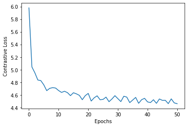
Figure 3: Contrastive training loss across training epochs.

A good feature representation is expected to generalize and perform well without additional training and fine-tuning. We examine this by freezing the feature network and only training a linear evaluator for classification. We achieve an accuracy of 71.3% on a small labeled dataset, while a randomly initialized model with the same setup only achieves 15.6%--showing that the learned representation actually performs well without the need for further training. Summary of all experiments are reported in Table 1.

	Full model (End-to-End)		Linear Evaluation (Frozen feature)
	Top-1 Accuracy	Top-3 Accuracy	Top-1 Accuracy	Top-3 Accuracy
SimCLR	77.4%	94.8%	71.3%	93.6%
Random Init	38.2%	60.1%	15.6%	34.4%

Table 1: Summary of experimental results.

Next, we inspect the feature-space clusters of the self-supervised representation networks by sampling random test images and finding nearest neighbor images in the feature space--after all, contrastive learning optimizes for maximizing similarity which should result in similar images being closer together. Figure 4 shows four random samples with the 5-NN images in feature space. Indeed we see that we managed to learn representations that cluster similar images, with some failure cases to note.

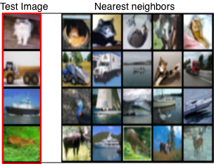
Figure 4: Nearest neighbors of test images.

Challenges

SimCLR is notorious for being compute intensive, requiring a large batch size as a way to ensure the availability of negatives which are essential for contrastive learning. The original paper uses 4096 batch size and trains for over 500+ epochs--our batch size tops at ~200, which immediately puts an upper limit on the maximum accuracy we can achieve. Despite this, we manage to demonstrate the capabilities of learned representation in the absence of large amounts of labeled data, albeit with a lower accuracy than the original paper.